
Effectiveness and optimization of bidirectional long short-term memory (BiLSTM) based fast detection of deep fake face videos for real-time applications
- Published
- Accepted
- Received
- Academic Editor
- Bilal Alatas
- Subject Areas
- Adaptive and Self-Organizing Systems, Artificial Intelligence, Data Mining and Machine Learning, Scientific Computing and Simulation, Neural Networks
- Keywords
- Deepfake detection, BiLSTM, Face video, Deep learning
- Copyright
- © 2025 Wang
- Licence
- This is an open access article distributed under the terms of the Creative Commons Attribution License, which permits using, remixing, and building upon the work non-commercially, as long as it is properly attributed. For attribution, the original author(s), title, publication source (PeerJ Computer Science) and either DOI or URL of the article must be cited.
- Cite this article
- 2025. Effectiveness and optimization of bidirectional long short-term memory (BiLSTM) based fast detection of deep fake face videos for real-time applications. PeerJ Computer Science 11:e2867 https://doi.org/10.7717/peerj-cs.2867
Abstract
This study proposes a rapid detection method for deepfake face videos designed for real-time applications using bidirectional long short-term memory (BiLSTM) networks. The aim is to overcome the limitations of current technologies in terms of efficiency and accuracy. An optimized BiLSTM architecture and training strategy are employed, enhancing recognition capabilities through data preprocessing and feature enhancement while also minimizing computational complexity and resource consumption during detection. Experiments were conducted on the FaceForensics++ dataset, which includes both authentic and four types of manipulated videos. The results show that the proposed BiLSTM-based approach outperforms existing methods in real-time detection. Specifically, the integration of temporal analysis and conditional random fields (CRF) resulted in significant accuracy improvements: a 1.6% increase in checking accuracy, a 2.0% improvement in checking completeness, and a 2.5% increase in the F1-score. The BiLSTM-based rapid detection approach demonstrated high efficiency and accuracy across multiple standard datasets, achieving notable performance gains over current technologies. These findings highlight the method’s potential and value for real-time deepfake detection applications.
Introduction
With the rapid development of multimedia technology, image and video processing methods based on deep learning have been greatly developed in recent years. In particular, the emergence of Deepfakes, which can generate realistic facial images and videos by using advanced machine learning models such as generative adversarial networks (GANs), has potential applications in entertainment, education and other fields. However, it also brings serious security and privacy issues (Zaynab & Hebah, 2022). As deep forgeries can be faked, this poses a threat to personal privacy and may also be used to create false information and cause social unrest. Therefore, how to improve the technology and efficiency of detecting and recognizing deeply forged content under the premise of security and privacy protection has become an urgent issue.
In the current research field, numerous innovative strategies have been proposed to recognize and detect fake face videos. These strategies cover from traditional feature analysis-based approaches to advanced methods using deep learning techniques. Ghai, Kumar & Gupta (2019) and others, in their research, worked on developing a deep learning-based architecture for image forgery recognition. Their proposed model specifically highlights the application of splicing techniques and copy-shift methods in the detection of forged images. Wang, Wang & Li (2019) proposed a new method that combines face feature point extraction with grey scale transformation. The algorithm improves the recognition efficiency by adjusting important features such as saliency, contrast, and complexity. Tao, Zhiguo & Yi (2021) proposed a new method that combines CNN with measure learning. They used a multiple hidden layer structure to extract deep features of the face. Hu et al. (2022) proposed a video analytics method for violence detection which deeply analyzes the video based on time series data and has high accuracy for real-time video detection.
In real-time detection of fake face videos, traditional methods face many challenges, mainly including:
(1) Efficiency problems: many existing techniques are slow in processing video streams and cannot meet the demands of real-time analysis.
(2) Insufficient accuracy: due to the increasing sophistication of forgery techniques, traditional methods make it difficult to capture subtle anomalies in the forged videos, resulting in low accuracy.
(3) High consumption of computational resources: some high-precision detection algorithms require a large amount of computational resources, which is not conducive to deployment on resource-constrained devices.
(4) Insufficient dynamic feature capture: video is dynamic, and traditional methods tend to focus on single-frame analysis, which makes it difficult to make effective use of time-series information.
To address these issues, this study proposes an improved method based on bidirectional long and short-term memory networks (BiLSTM) to increase the efficiency and accuracy of detection:
(1) Optimized BiLSTM model structure: with the improved model structure, the algorithm in this article is able to process video data more quickly and meet the demand of real-time analysis.
(2) Innovation of training strategy: a new training strategy is adopted to improve the model’s recognition accuracy of forged videos.
(3) Reduced resource consumption: the model optimization reduces the computational complexity and resource consumption in the detection process, making it more suitable for running on resource-constrained devices.
(4) Enhanced dynamic feature analysis: the bi-directional nature of BiLSTM enables the model in this article to better capture the dynamic changes and contextual information in the video, thus improving the detection accuracy.
The model proposed in this article has the following contributions:
In this study, we develop a fast detection method based on BiLSTM for deep forgery face videos for real-time applications. The method significantly improves the recognition ability and detection speed of the model by optimizing the model structure and training strategy, combining data preprocessing, feature enhancement techniques, and timing analysis, while reducing the computational complexity and resource consumption.
In this article, a fast detection framework based on BiLSTM is proposed for recognizing in-depth forged face videos, which improves the model’s recognition ability of forged content through data preprocessing and feature enhancement techniques and adopts a model optimization strategy, which effectively reduces the computational complexity and resource consumption in the detection process, and combines the Conditional Random Fields (CRF) technique with the optimization of the output of BiLSTM to improve the accuracy and reliability of the discrimination.
It is demonstrated through experiments that the BiLSTM-based method proposed in this article shows superior performance in real-time detection, and compared with the single-frame discriminative network Xception and the BiLSTM method without introducing CRF, the introduction of temporal analysis and CRF results in a significant improvement in the accuracy, check accuracy, check completeness, and F1 value and the experiments on multiple standard datasets validate that the proposed method has high efficiency and high accuracy in real-time detection with high efficiency and accuracy. Compared with the existing techniques, the method has significant performance improvement in detecting deeply forged videos, proving its potential and value in real-time applications.
Related work
BiLSTM, as a powerful sequence processing model, has received much attention in the field of deep forgery detection. It has been shown that BiLSTM can effectively capture dynamic features and contextual information in video content, thus improving the detection accuracy of forged videos. Lu, Tai & Tang (2018) converted low-quality images into high-quality ones by proposing CycleGAN, which finally generated high-quality deep forged videos. RSGAN (Natsume, Yatagawa & Morishima, 2018) achieves face swapping by separating the face part and the hair part into two different potential spaces for variational learning and then performing different processing on the potential spaces to achieve face swapping. Chhabra et al. (2023) propose a multi-channel null convolution module to improve the model’s detection accuracy on low-quality forged face videos; Li & Yu (2020) introduced noise flow features and designed a dual flow detection framework based on the EfficientNet model; Kumari & Durga (2024) proposed an improved ResNet network combined with data augmentation to enhance the model’s detection performance on two types of tampering, Deepfakes and FaceSwap. Kim et al. (2018) further improved the realism of the faked video by combining traditional 3D and generative adversarial network techniques to transfer expressions and gestures into the target object.
However, although BiLSTM performs well in sequence data analysis, it still has some limitations when dealing with deeply faked face videos. Firstly, BiLSTM models usually require a large number of parameters, which may lead to high computational costs in practical applications. Second, BiLSTM may encounter the problem of gradient vanishing or gradient explosion when dealing with long sequence data, which affects the training effect of the model. In addition, most of the existing BiLSTM-based deep forgery detection methods focus on the static characterization of video frames and ignore the information of dynamic changes between frames, which restricts the model’s ability to detect deep forgery videos.
This study aims to propose a fast BiLSTM-based deep forgery face video detection method for real-time applications by optimizing the BiLSTM model structure and training strategy and combining data preprocessing and feature enhancement techniques. The method in this article not only improves the speed and accuracy of detection but also reduces the computational complexity and resource consumption, thus demonstrating superior performance in real-time detection. Table 1 provides a comparison of methodologies in deepfake detection.
| Methodology | Strengths | Limitations | Key feature |
|---|---|---|---|
| Xception | High accuracy for static image classification | Struggles with temporal consistency across video frames | Focuses on frame-level analysis |
| MesoNet | Efficient for face image recognition | Limited temporal feature capture, not ideal for videos | Specializes in facial image analysis |
| Capsule networks | Effective at recognizing spatial relationships in images | Computationally expensive and struggles with real-time detection | Uses capsules to preserve spatial hierarchy |
| ConvLSTM | Captures temporal dependencies in video frames | High computational cost and may not perform well in real-time scenarios | Combines convolutional networks and LSTM |
| Proposed model (BiLSTM + CRF) | Captures both forward and backward temporal dependencies; improves prediction consistency across frames | Requires more data and computational resources for training | Uses BiLSTM for temporal analysis and CRF for frame consistency |
Methodology
Bidirectional long and short-term memory networks and deep falsification techniques
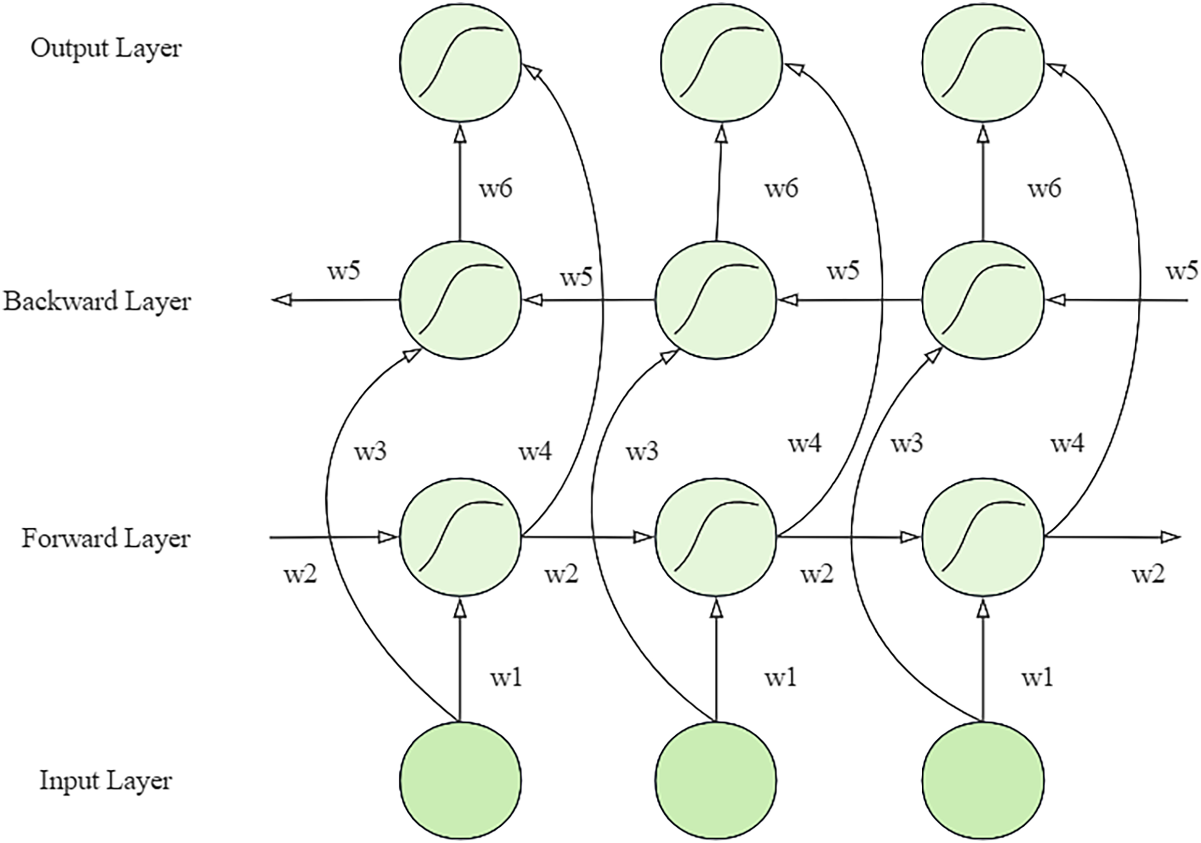
In the network structure of BiLSTM, the forward propagation layer and the backpropagation layer are its core components, as shown in Fig. 1. These two layers work together to produce the final output by sharing weights (Song et al., 2024). Specifically, the network performs forward operations through the forward propagation layer and records the state of the hidden layer at each time point. Then, the backward propagation layer oppositely performs operations, capturing information from backwards to forward. The outputs from these two directions are finally fused in the output layer to form a comprehensive prediction for each point in time. Two LSTM layers with forward and backward orientation form the model structure, which analyzes video sequences in different directions. Multiple layers produce their output, which gets combined to deliver an entire video understanding. The training process included multiple essential strategies that used advanced Xception features to boost BiLSTM performance at detecting fine details in video frames (Hu et al., 2023). Temporal dependencies of the BiLSTM network received optimization through the implementation of CRFs. Multi-task convolutional neural network (MTCNN), together with OpenCV, allowed precise face detection and frame extraction to ensure the model received only important data. The training incorporated both cross-entropy loss as well as auxiliary classifiers to enhance its learning speed and generalization capabilities. Strategies implemented in this approach have enhanced the deepfake detection capabilities of the model while keeping operational expenses minimal.
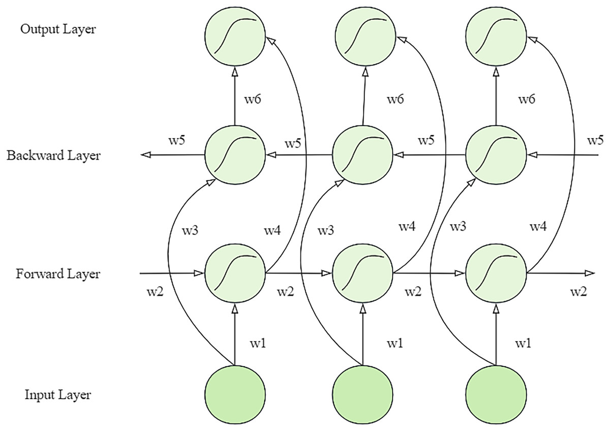
Figure 1: Structure of bi-directional LSTM network.
The network contains two conduction layers, forward and reverse, connected to the output layer and share six parameters (W1 to W6) (Agarwal & Verma, 2020). The network first performs forward computation through the forward layer to record the output at each step. Then, the reverse layer processes it to capture the reverse information. The final output is the sum of forward and reversed outputs. Its mathematical representation is shown below:
(1) (2) (3)
It contains the output of the forward propagation layer at time point , the output of the backward propagation layer at time point , and the output of the output layer at time point .
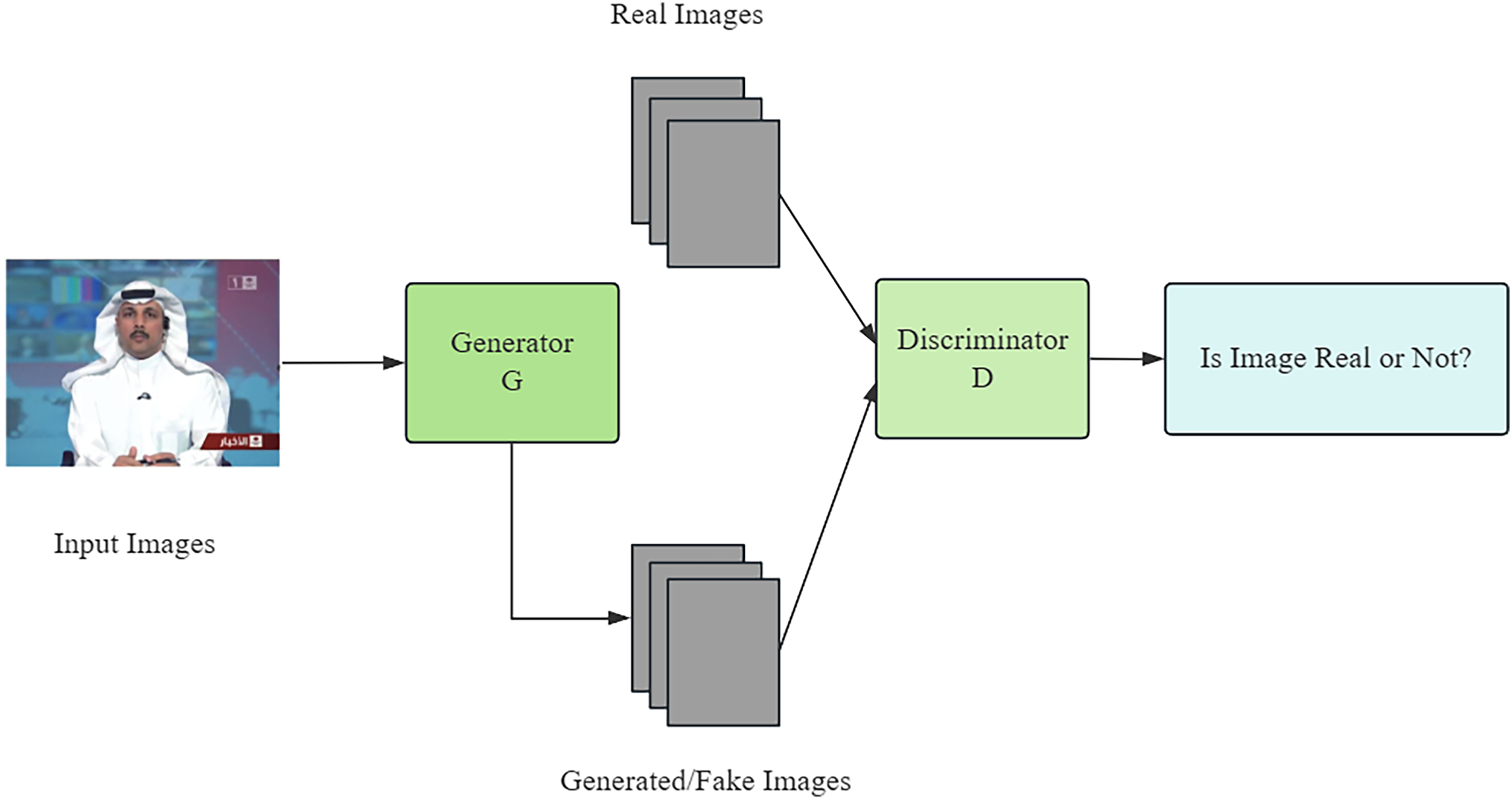
The core of deep forgery techniques is the generative adversarial network (GAN), which is constructed by two competing neural networks: a generator network, whose duty is to create realistic forgery data, and a discriminator network, whose core is to recognize these forgery data (Elaskily et al., 2021). In this process, the generator and the discriminator compete with each other through continuous iteration and optimization, and the generator network gradually improves the quality of the data it generates until it is difficult for the discriminator network to distinguish the authenticity. With the continuous advancement of technology, GAN can generate more realistic images and even deceive some advanced detectors (Samir, Youssef & Nagy, 2021). The branching structure of the GAN network is shown in Fig. 2.
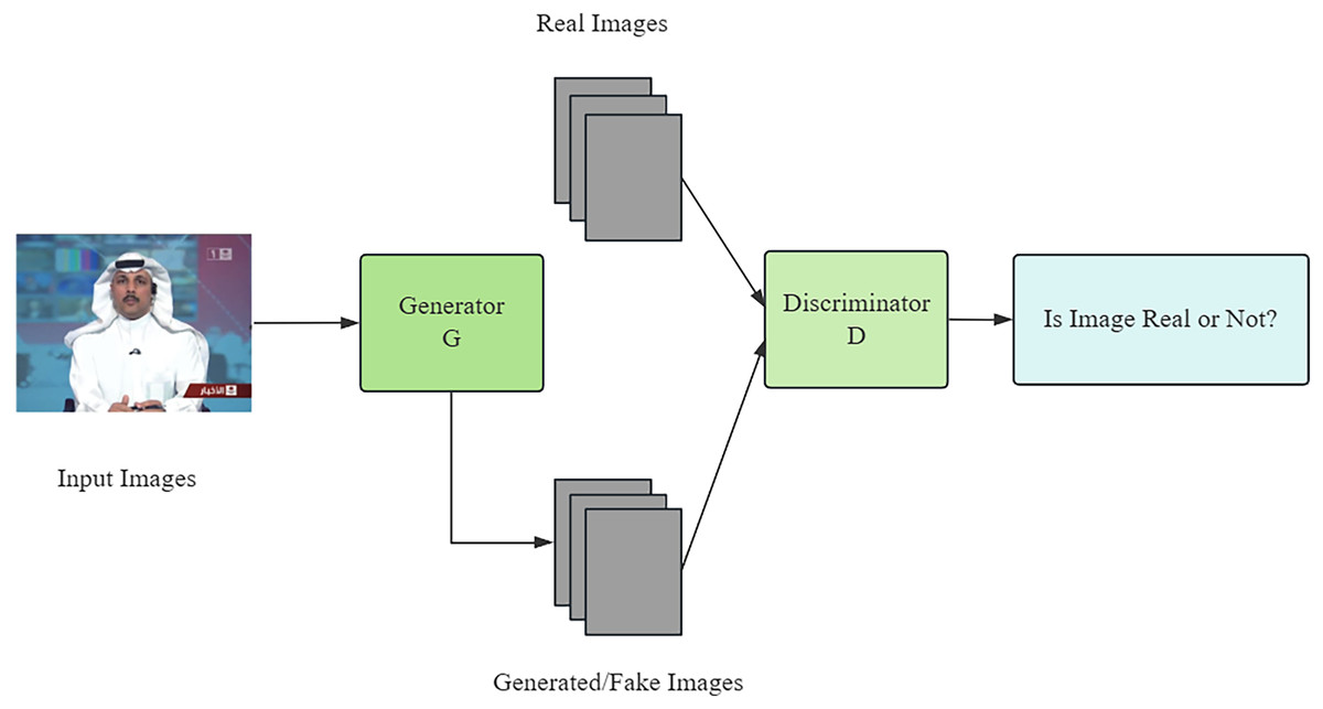
Figure 2: Framework diagram of GAN.
Combining the sequence processing capability of BiLSTM and the generative capability of GAN (Wang et al., 2023), the research in this article aims to develop a fast detection method for deeply forged face videos for real-time applications. The method improves the speed and accuracy of detection by optimizing the model structure and training strategy while keeping the computational cost low.
BiLSTM model architecture
BiLSTM fundamentals
The BiLSTM is an advanced sequence analysis model that combines the strengths of both forward and backward LSTM networks, resulting in bi-directional enhancements in data parsing. This design allows BiLSTM to capture and analyze sequence information from both forward and backward directions simultaneously, significantly improving the model’s ability to predict and understand information (Wang et al., 2022). LSTM functions as a specialized version of RNN because it serves as a sequential data processing model that enables the retention of extended temporal connections. The network maintains a cell state while its gating mechanisms control information flow through forgetting and input and output gates. LSTM features the ability to memorize important information across extended sequences, which proves valuable, particularly when analyzing videos where temporal frame connections matter (Hu et al., 2022). The capability of BiLSTM to examine a sequence from both forward and backward directions improves its video content understanding because it secures contextual information from previous and subsequent frames.
The efficient functioning of the LSTM network relies on the sophisticated structure within it, including the input at time step , the cell state , the hidden layer state , and the key forgetting gates , input gates , and output gates (Kumar et al., 2020).
The LSTM network computation process is shown in the following equation:
Calculate the oblivion gate:
(4)
Compute the memory gate:
(5) (6)
Calculate the current moment cell state:
(7)
Calculate the output gate and the current moment hidden layer state:
(8) (9) where are the respective weights, and are the offsets. The BiLSTM model architecture is shown in Fig. 3.
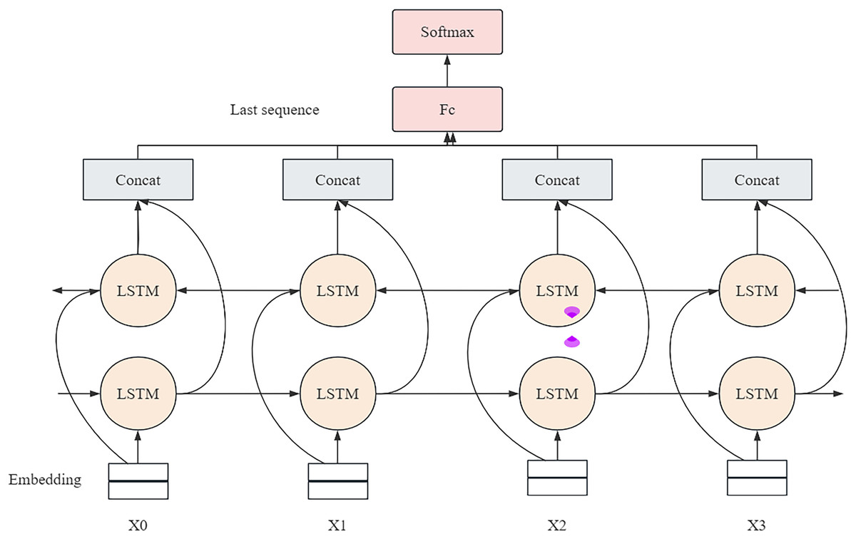
Figure 3: The model architecture of BiLSTM for deep forgery video detection.
Model design
This article uses a BiLSTM to capture the subtle differences of the forged video between the front and back frames. By starting from the video’s temporal characteristics, BiLSTM can deeply analyze and understand the dynamic changes in the sequence, thus revealing the timing anomalies of the forged video. Meanwhile, this study will also use the CRF technique to optimize the output of BiLSTM to improve the accuracy and reliability of the discrimination. A conditional random field is a new type of timing model that can achieve the precise adjustment of bilinear short-term memory by capturing the correlation in timing data and then improving the accuracy of the discrimination. The selection of BiLSTM for this work is due to its exceptional performance when working with sequential data, particularly video frames, in deepfake face video detection tasks. BiLSTM can spot interesting movement directions within a video series better than single-frame systems thanks to its ability to analyze both past and future frame connections. The technique shows its strength by analyzing two-directional data patterns to identify small frame differences that can reveal deepfakes. Besides having both high detection accuracy and productive speeds, BiLSTM supports shorter processing time for real-time deepfake checks on devices with limited bandwidth. The long-term memory capabilities of BiLSTM allowed us to choose it because deepfake video manipulation often occurs across multiple video frames.
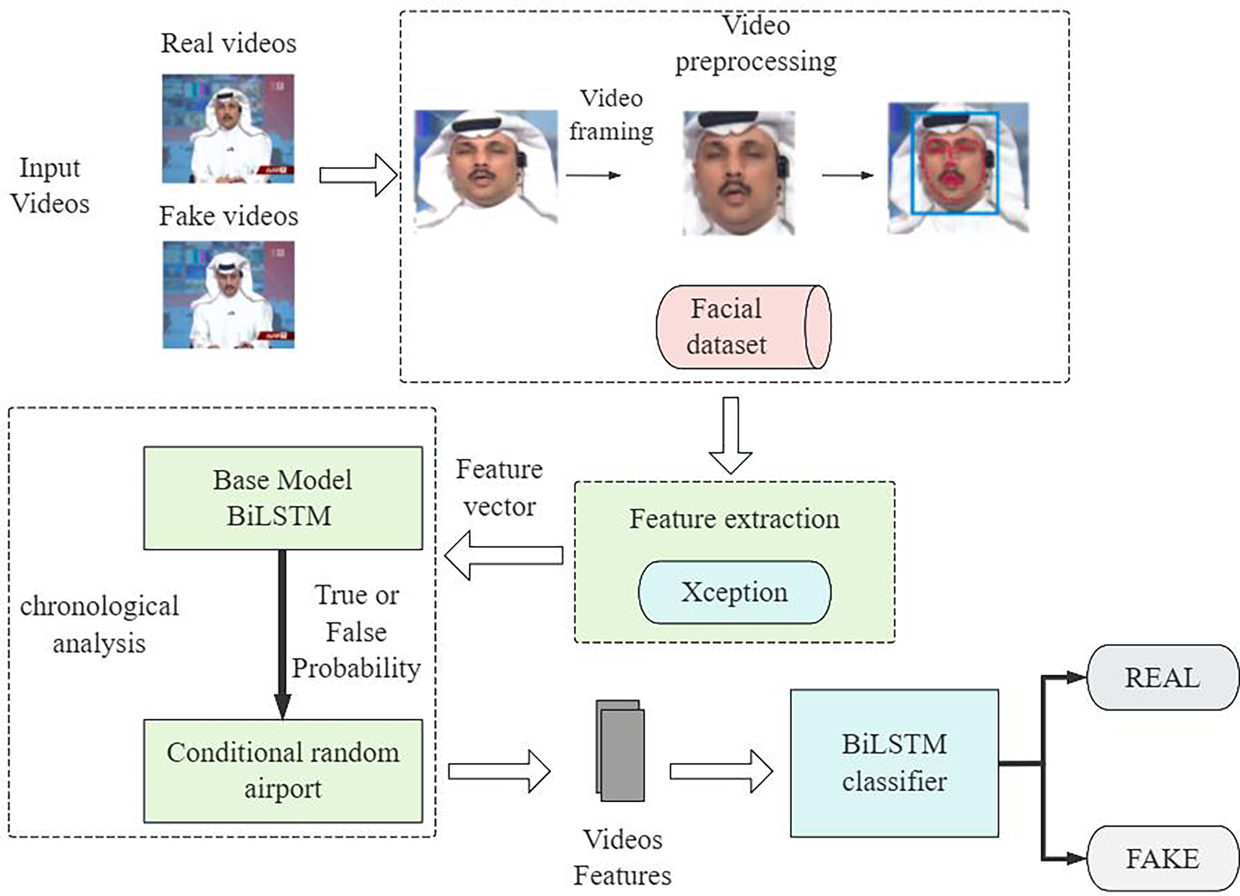
Figure 4 shows the overall architecture of the deep forgery video recognition proposed in this study, which integrates the timing analysis capability of BiLSTM and the sequence optimization technique of CRF to build a comprehensive set of detection strategies. The BiLSTM system processes video frames using its backward and forward dependency mechanism, yet Xception extracts the specific features. The CRF layer recognizes optimal temporal connections in BiLSTM outputs to maintain reliable predictions between successive video frames. This framework not only improves the detection accuracy of forged videos but also adapts to continuously updating forging techniques. It is versatile and adaptable.
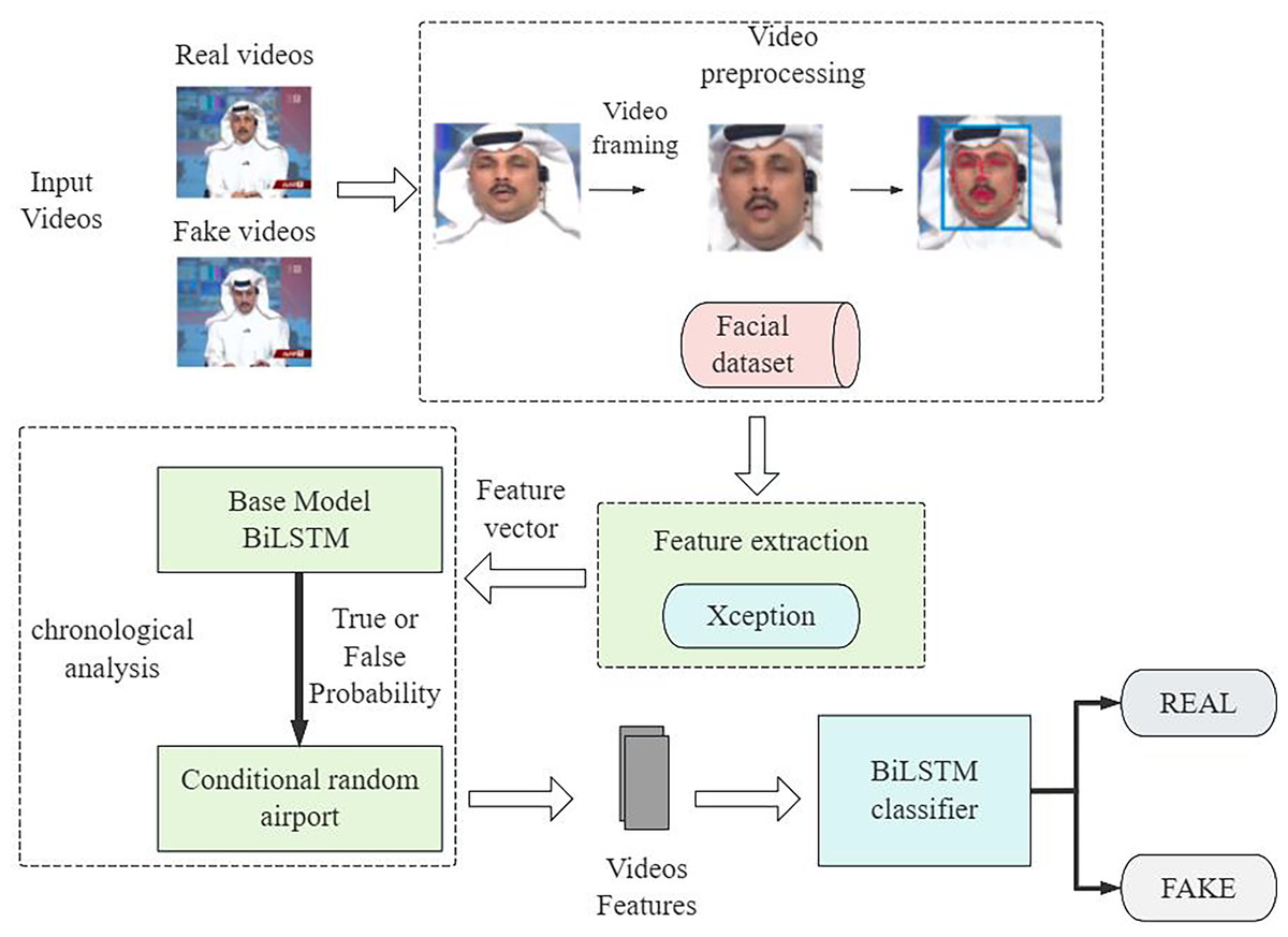
Figure 4: General framework of the model.
Feature extraction
In the video preprocessing phase, the research selected a series of image sequences and used them as inputs to the research’s video frame feature extraction module. During this period, the study utilized an advanced network structure based on Xception (Sharma, Sharma & Kalia, 2023), which is a modified model of Inceptionv3. Xception successfully captured the fine-grained information in the video frames by independently processing the channel and spatial dimensions while incorporating techniques from deeply separable convolutional and residual networks (Jaleed et al., 2018).
In order to optimize and maintain the appropriate number of covariates, deep segmented convolution was employed to enhance the modelling efficiency and quality of the study and based on the results of a series of comparative experiments done with the current major recognizers (e.g., MesoNet, MISLne, and Inception-v3), it can be ascertained that the Xception architecture has the best expressive power. It achieves a high level of recognition and effectively captures rich elements of the original image characteristics.
Based on this observation, the Xception network was selected as the basic framework for the study to obtain feature information, and it was set up and optimized in detail. After several rigorous training sessions, the study successfully obtained a feature vector of 2,048 dimensions after global mean pooling. The exquisite design of the Xception network, which consists of three main parts: the input stream, the mid-level stream and the output stream, allows the study to obtain all-round and in-depth feature information.
Finally, the study uses the extracted video frame feature vectors as inputs to the Bi-LSTM network in the subsequent temporal analysis phase in order to understand and analyze the video content in greater depth.
Timing analysis
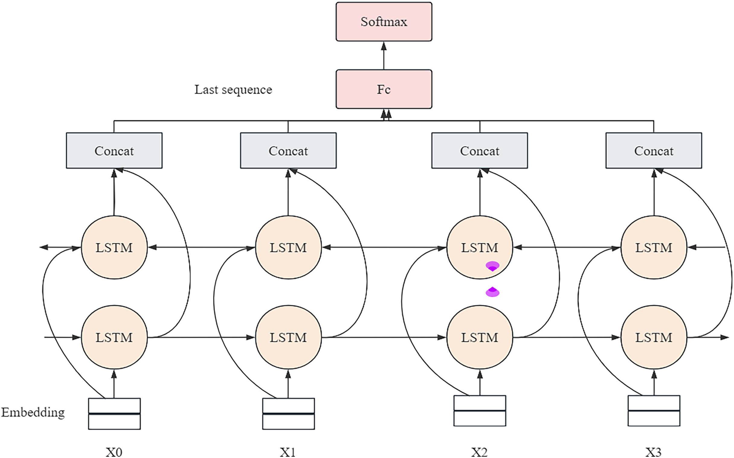
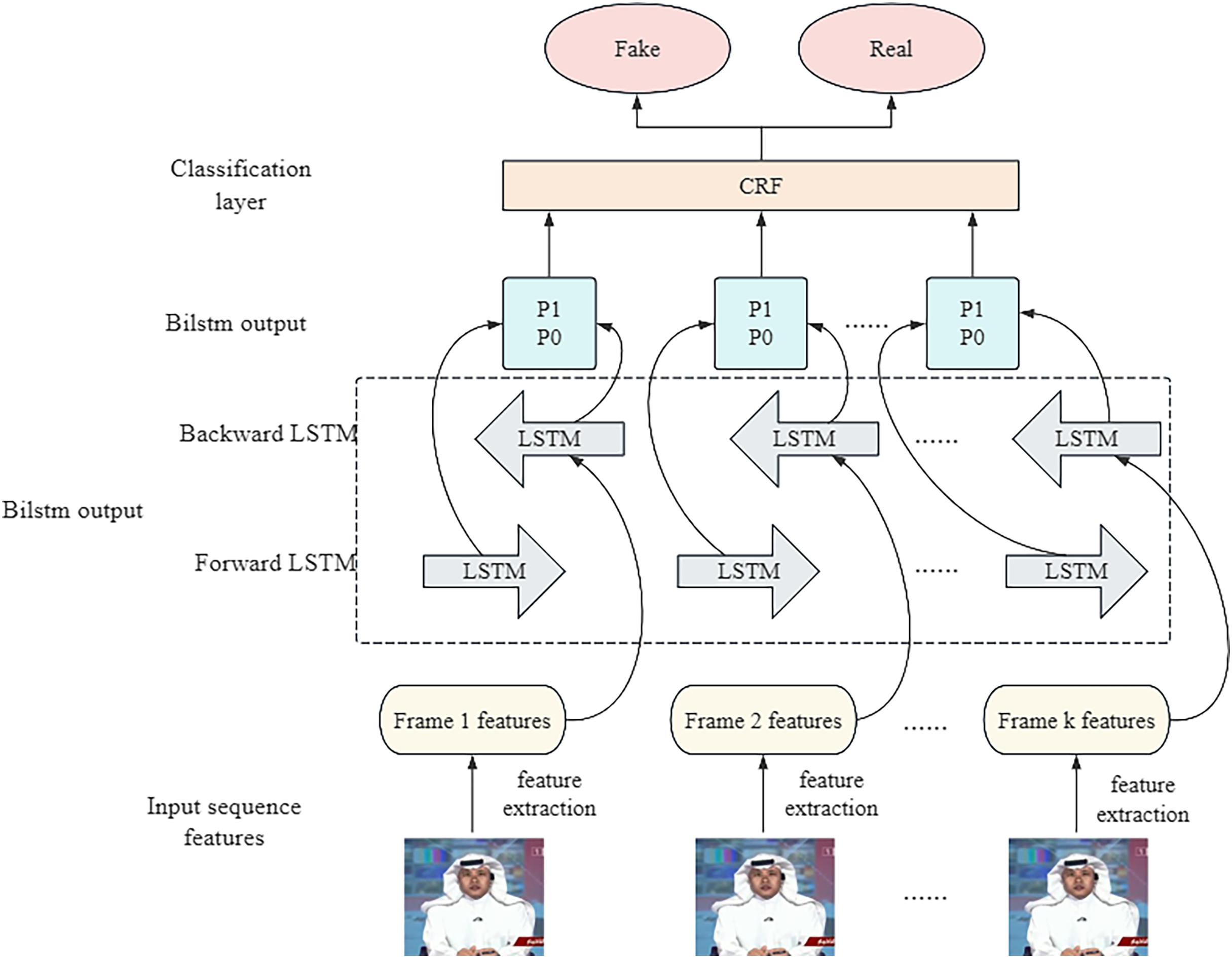
In the process of time series analysis, the model architecture adopted is shown in Fig. 5. The model takes the feature vector of the video frame sequence obtained in the feature extraction stage as the input. These feature vectors are then fed into a BiLSTM. In BiLSTM, the forward LSTM and the reverse LSTM operate independently and perform their computation processes separately.
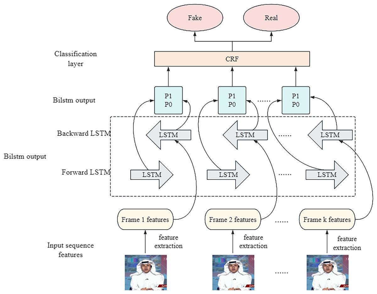
Figure 5: Timing analysis model.
Forward LSTM is responsible for the transmission of information from the beginning to the end of the sequence, capturing the forward dependencies in the time series. The reverse LSTM transmits information from the end of the sequence to the beginning in reverse order to capture backward dependencies. Through this bidirectional processing, the model can fully understand the dynamic changes in the sequence (Wu et al., 2023) and thus achieve more accurate and comprehensive predictions in time series analysis.
Processing data using the LSTM algorithm preserves key information and eliminates useless information, which helps in updating the state of each group of neuronal units (Xu, Park & Zhang, 2019). This allows long-distance correlations between feature vectors to be maintained, which in turn enables the feature vectors in consecutive frames to be combined with the contextual environment in which they are embedded for a deeper understanding of this inter-frame information. This information is then deeply mined using the BiLSTM technique, which finally gives the likelihood of the video being true or false in the form of a softmax function. Next, the study takes the independent probability values of the BiLSTM outputs as inputs into a CRF (Liu, Gao & Huang, 2021) model, and with the help of the model’s correlation characteristic function and transition probabilities, the study applies the Maximum Likelihood method of training, which yields the best possible output probability results.
Training strategies
Loss function
The measure is used to measure the size of the gap between the expected output result and the actual result from the input information, which is generally described by (Kumar & Kumar, 2018). The optimized neural network structure, when the value of its loss function is small, means that the expected output is closer to the real output, which represents a better performance of the network. Therefore, the whole learning process of the neural network is actually a method of finding the network parameters that can make the loss function optimal.
In this network model, the Softmax loss function is used for calculation, and the specific formula is shown below (Kim et al., 2018):
(10)
In Formula (10), represents the I-th sample, represents the corresponding label of the sample, represents the JTH column of the weight matrix of the last FC layer of the network, and represents the bias matrix of the last fully connected layer. N and m represent the size and total number of categories of small batch samples, respectively. The BiLSTM model employs the commonly used cross-entropy loss function as its loss function during deepfake detection classification. The function evaluates the difference that exists between forecasted probability values and actual video frame labels. Training the model struggles to achieve minimal loss through the cross-entropy loss function, which checks how accurate predictions mirror actual labels. Then, the inclusion of an auxiliary classifier loss to enhance model generalization along with speeding up its training convergence. The auxiliary loss operates jointly with the main loss functions to help models gain a better understanding of intricate video features within the dataset. The use of multiple loss components within the model enables better accuracy in detecting deepfakes alongside optimal performance through reduced overfitting.
In order to speed up the training of the network, an additional auxiliary classifier is added to the network structure, and the final loss function consists of the main classifier loss function and the cross-entropy loss function, which is calculated as shown below.
(11)
Specifically, the loss function in Formula (11) introduces two key components: the auxiliary classifier loss function and the cross-entropy loss function . Here, represents the characteristics of the input sample , while represents its six category labels. Additionally, and represents the predicted values of the deep network and auxiliary classifier respectively. denotes the parameters of the network, and is the weight factor for the auxiliary classifier loss in total loss. Furthermore, to enhance model generalization and prevent overfitting, a regularization term is added to control model complexity and ensure high discrimination accuracy with new data.
Optimizing mechanism
After the application of BiLSTM processing, the representation of the data distribution in the neural network may change (Sivakumar, Sasikumar & Krishnamurthy, 2023). To solve this problem, the batch normalization technique is used to adjust the learning environment of deep neural networks. This method can accelerate the training process of deep neural networks, and ensure the learnability and stability of the network. In this way, the distribution consistency of input data can be maintained and significant fluctuations of nodes within the network can be avoided. Using Batch Normalization can effectively improve the convergence rate of the network and maintain the performance of the neural network. The specific calculation process is as follows:
(1) Calculate batch mean and variance: for each layer of input , first calculate the mean and variance of the current batch (mini-batch).
(12)
(13)
(2) Normalization: the input is then normalized using the batch mean and variance to obtain
(14) where is a very small constant used to ensure numerical stability.
(3) Scaling and panning: the normalized input is scaled and panned by two learnable parameters, which are (scaling factor) and (panning factor).
(15) where y is the output after normalization, scaling, and translation. During training and the operational run of the BiLSTM model, the optimization mechanism functions as a vital element. It performs optimization through the batch normalization approach. The normalization technique prevents unstable training conditions because it controls input data flow through each neural network layer. The learning process remains unhindered by internal covariate shifts because the normalization technique is implemented. The model becomes less sensitive to learning rate changes through batch normalization because this technique normalizes activation values in each layer. Relevant to overfitting prevention, it implements a regularization force that adds slight noise to training operations. When batch normalization operates with optimized hyperparameters, it helps the model learn efficiently and acquire the ability to generalize to data that was not used during training. The optimization mechanism optimizes model performance, which allows it to handle large-scale video data effectively with enhanced detection accuracy and robustness of deepfake content.
Detection optimization strategies
The technique of combining BiLSTM with CRF provides a highly efficacious analytical tool in the field of sequence analysis (Chakraborty, Bhattacharyya & Ghosh, 2023). The predictions from BiLSTM benefit from CRF because they model the logical connections between successive video frames. CRF serves as a sequentially structured model because it evaluates each frame output through input information from the present time and neighbouring frame labels. Using CRF allows the production of consistent predictions throughout adjacent frames, thus enhancing video classification accuracy. CRF enables better temporal consistency in predictions through our study, which leads to increased model performance when detecting deepfake videos. The output of BiLSTM after being used for temporal analysis is the probability corresponding to each label. Further accessing the results after BiLSTM is done with a conditional random field, the results are optimized by the conditional random field to get the final identification result. The detection optimization approaches analyze two aspects of deepfake face video detection: accuracy rates alongside operational speed. A vital detection strategy consists of implementing CRF together with BiLSTM networks. By implementing CRF, the model becomes better at identifying real or fake videos through frame context analysis. The Xception network optimizes feature extraction by capturing detailed aspects of video frames to detect faint discrepancies in the content. The training process becomes more stable after implementing the batch normalization technique, which promotes faster convergence and minimizes both speed-related problems. The combination of these techniques enhances model accuracy and computational efficiency, thus enabling it to perform continuous video detection operations efficiently. CRF is a serialized labelling algorithm that finds the corresponding variable under a given condition. Given two random variables , and is the given condition, if the random variable constitutes a Markov random field that can be obtained from an undirected graph , i.e., for any node in the undirected graph such that Formula (16) holds:
(16)
In an undirected graph , represents the set of vertices and represents the set of edges. CRF is a statistical modelling approach for working with structured data, where denotes the probability of output given input . In a CRF model, each vertex is associated with a set of vertices connected to it that do not include itself.
The CRF model captures the characteristics of the data by defining a feature function. For example, for input , the feature function can describe the relationship between the state at the current position and the state at the previous position . This feature function allows the model to take into account information from neighbouring data points when classifying.
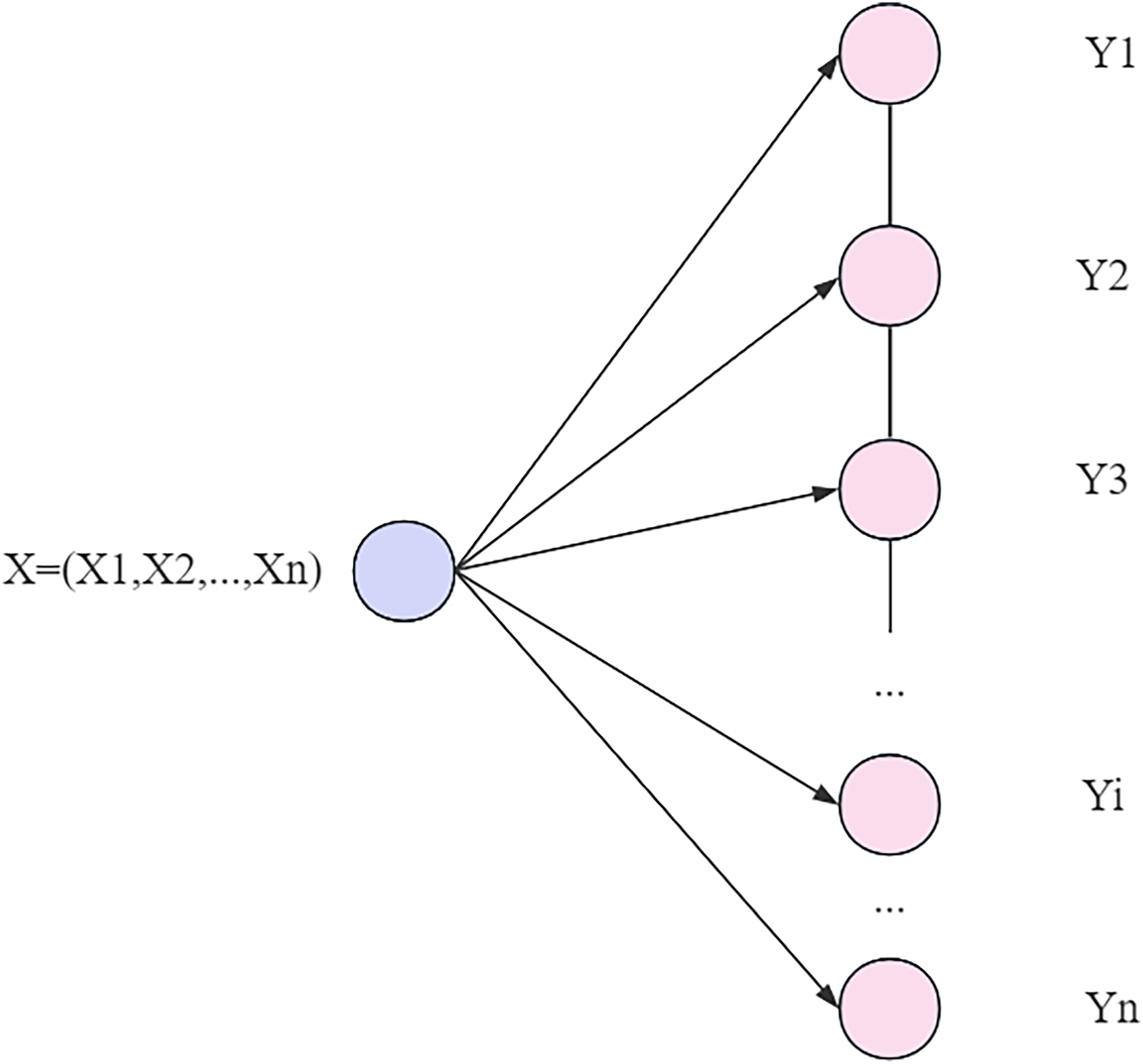
In CRF implementations, linear conditional random fields (LCM) are a common form. In the training phase, the LCM uses maximum likelihood estimation (MLE) or regularized MLE to learn the model parameters in order to predict the output sequence corresponding to the input sequence. In this way, the CRF model is able to effectively classify and label the input data while taking into account the interrelationships between data points. As shown in Fig. 6, the goal of the training process is to find model parameters that maximize the likelihood of the training data.
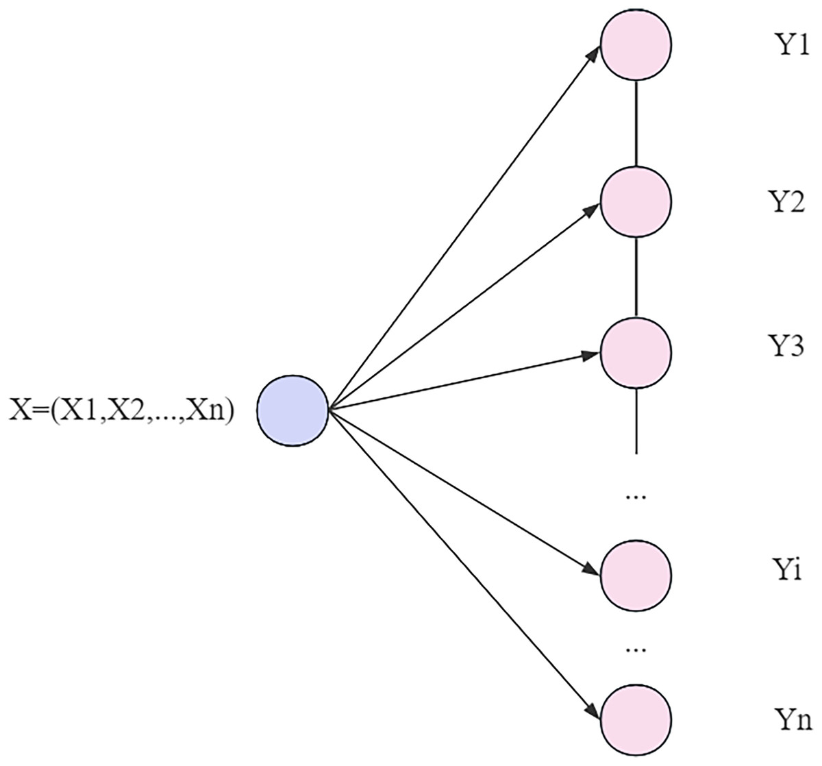
Figure 6: Linear chain conditional random field.
LCM (He et al., 2019) feature functions are classified into two categories: one is the nodal feature function that depends only on the current node, where a range from 1 to , where represents the number of nodal feature functions defined on the node , and represents the position of the current node in the sequence. The other class is the local eigenfunctions that depend on the current node and its predecessor, where b ranges from 1 to B, where B represents the number of all local eigenfunctions defined on the node, and i−1 represents the position of the previous node in the sequence.
In calculating the probability of a conditional random field it is actually a process of calculating the conditional probability and its mathematical expectation given the input sequence and output conditions. This calculation can be expressed as the product of the mathematical expectation function and the normalization factor. Essentially, a conditional random field is a log-linear model defined on time-series data, and its training process involves a log-likelihood function, as shown in Eq. (17).
(17)
After processing by a BiLSTM network, a series of predicted values of video frames can be obtained. These predicted values are fed into a conditional random field, where the constraint relationships between the predicted values are automatically learnt through transfer matrix operations and the model is trained using maximum likelihood methods to reduce the error rate. For example, when a set of video sequences with feature vectors are fed into a BiLSTM network for analysis, each vector produces a set of predicted values . The conditional random field learns the predicted values of each globally through a transfer matrix. It selects the best set of predicted values as the prediction result of the current sequence features, thus obtaining the optimal prediction result of the whole video frame sequence.
Experiment
Dataset and preprocessing
In this experiment, the study used the FaceForensics++ database, covering 1,000 source face videos posted on YouTube, where each segment is in the range of 10 to 15 s in duration. These face videos were faked using four unique methods: Deepfakes, FaceSwap, Fac2Face, and NeuralTextures. Deepfakes and FaceSwap focus on identity transformation, while Fac2Face and NeuralTextures work on facial expression reenactment. The research employed fake video content in greater numbers than real videos because deepfake detection tasks typically deal with unequal data ratios. Creating fake videos requires the production of an extended quantity of artificially generated content as opposed to real video material. The usage of additional fake images created opportunities for the model to discover subtle distinctions between authentic and counterfeit videos. Machine learning tasks often require this approach to benefit from a broad sample of training examples, particularly in cases where multiple manipulation detection situations are present in different datasets.
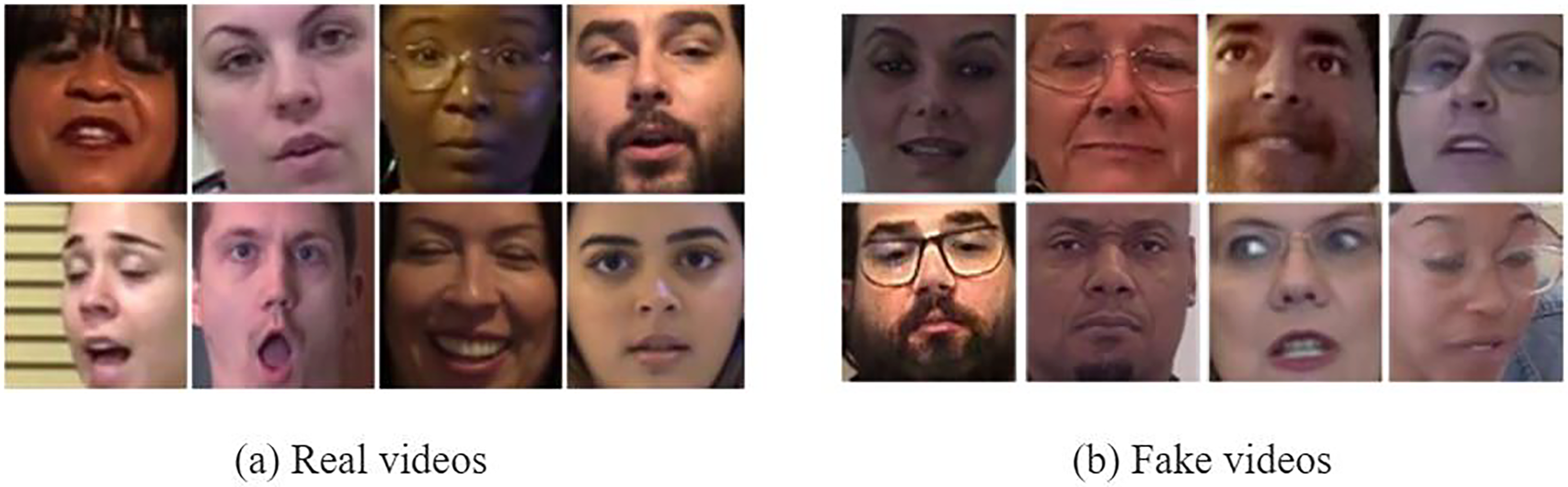
The experimental design of this study includes 1,000 real video samples and 500 videos for each of the four forgery techniques for the training and testing phases. All videos were processed with high-quality standards, as evidenced by a constant rate quantization parameter of 23, which ensures a clear and detailed representation of the videos. Some selected samples of the dataset are shown in Fig. 7, which not only demonstrates the diversity of the dataset but also reflects the rigour and depth of the experiments.
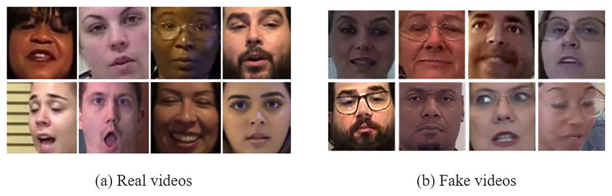
Figure 7: (A and B) Sample FaceForensics++ dataset.
The study adopted a systematic sampling method to ensure the randomness and fairness of the experimental results. From 1,000 real videos and 500 videos generated by each of the four forgery techniques, the study uniformly selected 30 frames from each frame. Such a sampling strategy ensured that the study’s dataset remained representative and diverse in all situations (Yu et al., 2023).
Next, the study divided these frame images into a training set and a test set in a ratio of 7:3. Specifically, the training set contained 21,000 frame images from the real video and 42,000 frame images from the fake video. In comparison, the test set contained 9,000 frame images from the real video and 18,000 frame images from the fake video.
Video preprocessing
In the journey of identifying deeply forged face videos, the study first performs a well-designed video preprocessing step to ensure the accuracy and efficiency of the subsequent analyses:
Video labelling and frame extraction: the study clearly labelled the videos in the dataset, with 0 for deeply faked videos and 1 for real videos. Subsequently, with the power of Python’s opencv library, the study smoothly divided the videos into consecutive frames and saved them properly.
Face detection method selection: before entering the face interception stage, the study conducted a careful comparative analysis of two face detection methods, Dlib and MTCNN. The results show that MTCNN outperforms Dlib in both detection accuracy and speed, especially when dealing with faces with different skin colours; MTCNN demonstrates excellent performance and maintains high accuracy even in the detection of faces with black skin colour (Yao et al., 2018).
Face interception: given the combined advantages of MTCNN in face detection and keypoint localization, the study chose this method for fast and efficient interception of face regions.
Image saving: the study saved the intercepted consecutive face images in the original order of the videos in the dataset. In order to meet the demands of subsequent processing, all saved images were uniformly resized to 256 × 256 pixels to ensure consistency and ease of processing (Elaskily et al., 2020).
Experimental setup
The experiments were performed on a device equipped with an Intel Core i7-6000 processor, a processor frequency of 3.40 GHz, and 8 GB of video memory. In this process, the Python language and NumPy library were used to perform matrix computation tasks, and the TensorFlow framework was used to develop and optimize the convolutional neural network on the back end.
In the parameter configuration part of the experiment, the FaceForensics++ dataset is selected as the research object, and two core parameters are particularly concerned: batch size and convolutional kernel size.
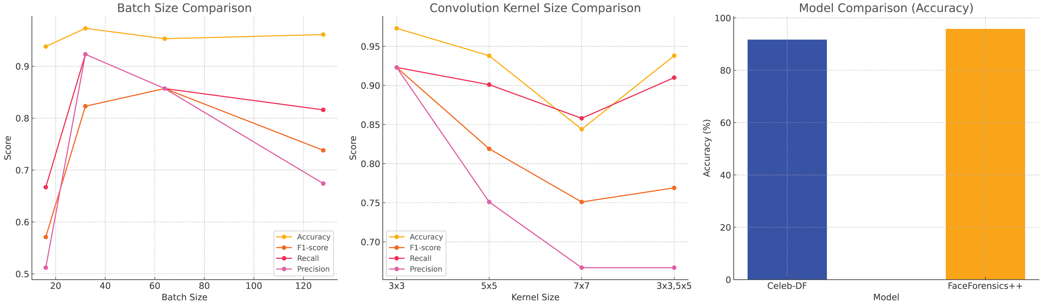
Choosing the right batch size is crucial to ensure the accuracy of the gradient descent algorithm and improve the efficiency of model training. A reasonable batch size can enhance the memory ability of the model for training data and accelerate the learning speed. However, if the batch size is set too low, it may cause the loss of training sample diversity and affect the generalization performance of the model. On the other hand, large batch sizes can lead to unnecessary consumption of computing resources. Therefore, balancing the choice of batch sizes is critical to achieving effective model training. Table 2 provides data on the effects of different batch sizes on model performance, with bolded values representing the best performance. In particular, when the batch size is set to 32, the recognition rate of the model reaches the highest value, so 32 is chosen as the batch size for training.
| Convolution kernel size | 3 * 3 | 5 * 5 | 7 * 7 | 3 * 3, 5 * 5 |
| Acc | 0.973 | 0.938 | 0.844 | 0.938 |
| F1-score | 0.923 | 0.819 | 0.751 | 0.769 |
| Recall | 0.923 | 0.901 | 0.858 | 0.910 |
| Precision | 0.923 | 0.751 | 0.667 | 0.667 |
The size of the convolution kernel directly affects the size of the output feature map. In theory, smaller convolution kernels are preferred, but when dealing with particularly sparse data, smaller convolution kernels may not adequately capture its features. Larger convolution kernels can capture more complex features, but they also increase the complexity of the model. Therefore, it is necessary to select an appropriate convolution kernel size. Table 3 shows the evaluation results of face recognition performance under different convolution kernel sizes, among which the convolution kernel size of 3 × 3 provides the best recognition effect. Hence, the study chooses 3 × 3 as the convolution kernel size.
| Batch size | 32 |
| Learning rate | 0.01 |
| Optimizer | Adam |
| Pooling size | 2 * 2 |
| Activation functions | ReLu |
| Loss functions | Cross-entropy loss function |
| Kernel size | 3 * 3 |
When constructing a convolutional neural network (CNN), in addition to batch size and convolutional kernel size, there are several key parameters to consider, including learning rate, optimizer selection, pooling layer size, activation function, loss function, and kernel size. Through iteration and optimization of a series of experiments, the optimal configuration of these parameters was set in the study, as shown in Table 4. These carefully selected parameter settings ensure the model can perform best during training.
| Model | Celeb-DF | FaceForensics++ |
|---|---|---|
| Meso4 | 54.8 | 84.7 |
| Capsule | 57.5 | 96.6 |
| ConvLSTM | 79.8 | 92.7 |
| DenseNet | 84.0 | 94.0 |
| The proposed model | 91.7 | 95.8 |
Performance evaluation
This research is devoted to solving the binary classification problem, aiming to distinguish the authenticity of a video by evaluating the detection probability, that is, to judge whether the video is real or has been deeply falsified. In order to comprehensively evaluate the validity of the proposed identification method, Accuracy is mainly used as the measurement standard. The calculation method of accuracy rate is described in detail by Formula (18).
(18)
The accuracy rate combines the following four key metrics (Thies, Zollhofer & Nießner, 2019).
In order to deeply analyze the impact of BiLSTM combined with conditional random fields and the convolutional block attention module introduced in the feature extraction phase on the discrimination effect, the study also used several other evaluation metrics, including precision, recall and F1 value. The precision rate, also known as the checking rate, refers to the proportion of correct predictions among all videos predicted to be deep forgeries, which is calculated as shown in Formula (19):
(19)
The recall rate, also known as the check-all rate, indicates the proportion of all actual depth-falsified videos that are correctly predicted and is calculated as shown in Formula (20):
(20)
Given that high precision and low recall, or vice versa, may occur in the actual identification process, the study introduces the F1 value to consider precision and recall together. The F1 value is the reconciled average of precision and recall, providing a single metric that balances the two, and is calculated as shown in Formula (21):
(21)
Analysis of experimental results
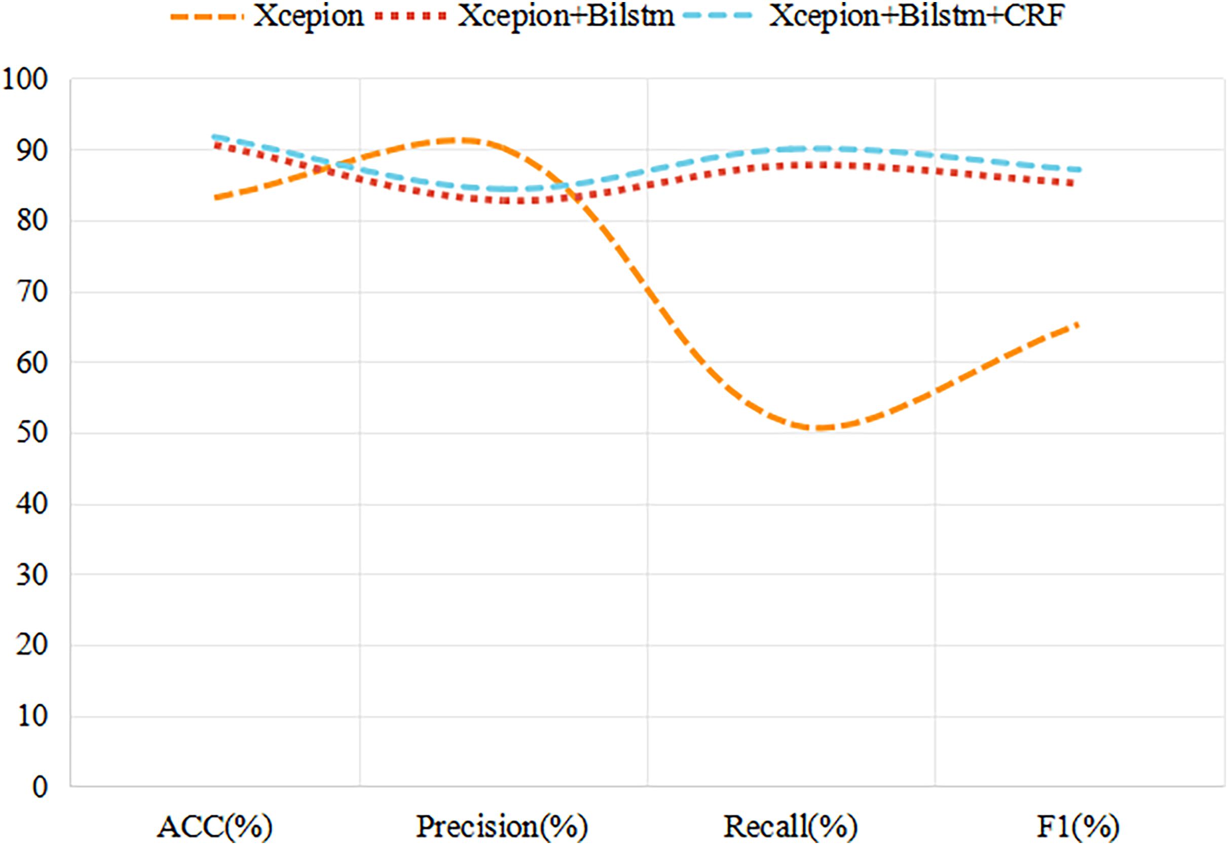
In this study, we develop a novel video discrimination technique that is grounded in the temporal inconsistency between video frames. Using a BiLSTM network, we are able to effectively capture inter-frame variations caused by depth forgery techniques, such as light source and resolution inconsistencies. To verify the effectiveness of our method, we compare its experimental results with the Xception network based on single-frame discrimination and the BiLSTM network without incorporating CRFs, and the experimental results are presented in Fig. 8.
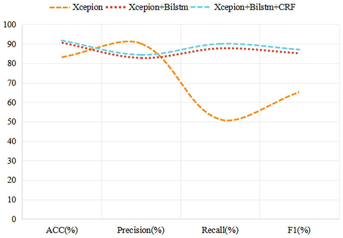
Figure 8: Experimental results for different network structures.
As can be seen from Fig. 8, time series analysis is more effective than the traditional single-frame recognition algorithm in improving the accuracy of recognition of deeply tampered videos. Moreover, when CRF processing is applied to the output of BiLSTM, the accuracy of the model is improved by almost 1%. Although the precision (Precision) is not the highest, it also achieves a 1.6% increase compared to the BiLSTM-only approach. Meanwhile, recall (Recall) and F1-scores performed the best among the compared methods, reaching 90.00% and 87.09%, respectively, and these results further confirm the effectiveness and superiority of the discriminative approach combining BiLSTM and CRF.
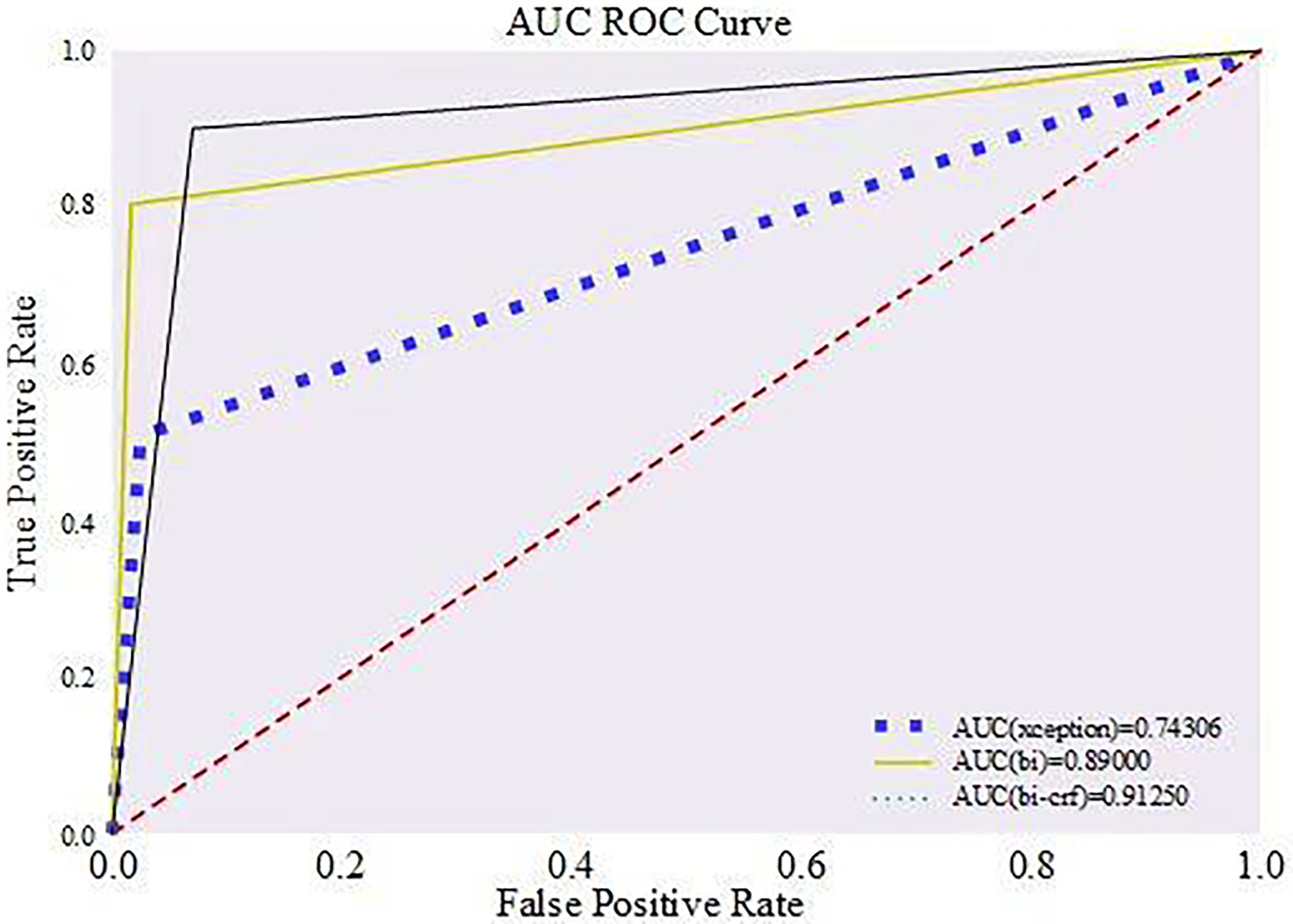
In order to show the correctness of the method more clearly, the ROC curve was drawn based on the true positive rate and false positive rate, as shown in Fig. 9. The dotted red line in the chart is used to rate performance. At the same time, the area below (AUC) is set at 0.5, representing the accuracy of random guesses.
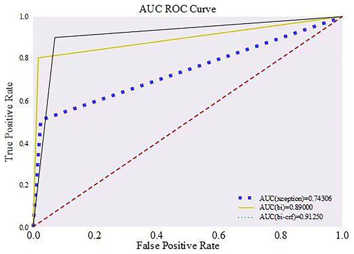
Figure 9: Comparison of ROC curves of different detection methods.
Located in the region above this baseline, the AUC value extends from 0.5 to 1.0, and a curve falling within this interval indicates that the identification method exhibits high accuracy and good performance. This is because a high AUC value means that the model can achieve a high rate of true positives at a lower rate of false positives. The region below the baseline, on the other hand, has AUC values ranging from 0.0 to 0.5, and a curve falling in this interval reflects a poor performance of the discriminative method, which has little value for practical application. The closer the AUC value is to 1 and the closer the curve is to the upper left corner, the better the classifier’s performance, which suggests that the model can effectively discriminate between positive and negative cases at all possible classification thresholds.
As shown in Fig. 9, the green solid line clearly presents the identification method proposed in this study that combines a LSTM with a CRF; the yellow line represents a BiLSTM-based identification technique that does not include a CRF; whereas the blue rectangular dashed line demonstrates an identification strategy that does not involve temporal analysis, i.e., it directly utilizes features extracted from Xception networks scheme for authenticity judgement through the fully connected layer. Comparing the data in Fig. 9, our discriminative method leads with an AUC value of 0.912, showing superior performance over the other two methods; followed by the discriminative method using only BiLSTM with an AUC value of 0.890, while the discriminative strategy employing the Xception network has the worst performance in terms of the AUC value, which is only 0.743.
This result is due to the strength of the LSTM network in capturing temporal inconsistencies between video frames and the role of the CRF in optimizing sequence classification accuracy. In contrast, the BiLSTM-only approach, although it also exploits timing information, does not have the global optimization capability of CRF, while the Xception network-only approach cannot analyze timing, resulting in a poorer performance in terms of AUC values than the one combining LSTM and CRF.
Combining the table and ROC graphs, the method proposed in this article achieves an improvement in deepfake video identification. In order to further validate the effectiveness of the method, the study also conducts comparison experiments between it and some of the current popular identification methods. The performance of the method in this article is evaluated against other methods mainly through the accuracy rate. Since the main current identification methods focus on single-frame identification and use datasets with obvious traces of forgery, we conducted comparison experiments on Celeb-DF and FaceForensics++ datasets, respectively.
After a comparative analysis, the method proposed in this study, which has the best performance on the Celeb-DF database, achieves a recognition accuracy of up to 91.72%. Although the method in this study did not achieve the optimal recognition on the FaceForensics++ database, there is only a 0.77% difference compared to the optimal recognition using the Capsule network (i.e., 96.60%). Therefore, the method proposed in this study achieves better detection results on both datasets and improves the detection rate of deeply forged videos. Figure 10 shows the overall comparison of the results. Similarly, Table 5 compares deepfake detection methods.

Figure 10: Comparison of various model and hyperparameter configurations, showing the impact of batch size, convolution kernel size, and model performance on deepfake detection accuracy.
| Methodology | Strengths | Limitations | Key features | Accuracy (Celeb-DF) | Accuracy (FaceForensics++) |
|---|---|---|---|---|---|
| Xception | High accuracy for static image classification | Struggles with temporal consistency across video frames | Focuses on frame-level analysis | 54.8% | 84.7% |
| BiLSTM (No CRF) | Captures temporal dependencies, better than frame-level methods | Lacks optimization for inter-frame consistency | Sequential data processing with LSTM | 57.5% | 96.6% |
| Capsule networks | Effective at recognizing spatial relationships in images | Computationally expensive, struggles with real-time detection | Uses capsules to preserve spatial hierarchy | 79.8% | 92.7% |
| ConvLSTM | Captures temporal features across frames | High computational cost, may not perform well in real-time scenarios | Combines convolutional networks and LSTM | 84.0% | 94.0% |
| DenseNet | High accuracy, effective feature reuse | Requires substantial computational resources | Dense connectivity of layers | 91.7% | 95.8% |
| Proposed model (BiLSTM + CRF) | Captures both forward and backward temporal dependencies; improves prediction consistency across frames | Requires more data and computational resources for training | BiLSTM + CRF for frame consistency | 91.7% | 95.8% |
Conclusion
In this study, we have successfully developed a fast detection method for deep forgery face videos based on a BiLSTM for real-time applications. Through well-designed model structure optimization and training strategies, combined with data preprocessing and feature enhancement techniques, our model significantly improves the speed and accuracy of detection while maintaining a low computational cost. Experimental results show that the method achieves efficient and highly accurate real-time detection on multiple standard datasets, demonstrating significant performance improvement over existing techniques.
Future work will further explore more efficient model optimization strategies and more advanced feature extraction techniques to continuously improve the performance and application scope of deep forgery detection. In addition, this study will focus on the generalization ability of the model under different forgery techniques and explore the performance of larger datasets.