
Ship detection based on semantic aggregation for video surveillance images with complex backgrounds
- Published
- Accepted
- Received
- Academic Editor
- Bilal Alatas
- Subject Areas
- Computer Vision, Artificial Intelligence
- Keywords
- Image processing, Ship detection, Semantic aggregation, Feature fusion, Video surveillance images
- Copyright
- © 2024 Ren et al.
- Licence
- This is an open access article distributed under the terms of the Creative Commons Attribution License, which permits using, remixing, and building upon the work non-commercially, as long as it is properly attributed. For attribution, the original author(s), title, publication source (PeerJ Computer Science) and either DOI or URL of the article must be cited.
- Cite this article
- 2024. Ship detection based on semantic aggregation for video surveillance images with complex backgrounds. PeerJ Computer Science 10:e2624 https://doi.org/10.7717/peerj-cs.2624
Abstract
Background
Ship detection in video surveillance images holds significant practical value. However, the background in these images is often complex, complicating the achievement of an optimal balance between detection precision and speed.
Method
This study proposes a ship detection method that leverages semantic aggregation in complex backgrounds. Initially, a semantic aggregation module merges deep features, rich in semantic information, with shallow features abundant in location details, extracted via the front-end network. Concurrently, these shallow features are reshaped through the reorg layer to extract richer feature information, and then these reshaped shallow features are integrated with deep features within the feature fusion module, thereby enhancing the capability for feature fusion and improving classification and positioning capability. Subsequently, a multiscale object detection layer is implemented to enhance feature expression and effectively identify ship objects across various scales. Moreover, the distance intersection over union (DIoU) metric is utilized to refine the loss function, enhancing the detection precision for ship objects.
Results
The experimental results on the SeaShips dataset and SeaShips_enlarge dataset demonstrate that the mean average [email protected] ([email protected]) of this proposed method reaches 89.30% and 89.10%, respectively.
Conclusions
The proposed method surpasses other existing ship detection techniques in terms of detection effect and meets real-time detection requirements, underscoring its engineering relevance.
Introduction
With the growth of inland waterway shipping, the complexity of inland waterway navigation environments has increased. The detection of inland waterway ships is crucial for ensuring their navigation safety and monitoring illegal fishing (Shao et al., 2018). This topic has attracted significant attention in the field of computer vision. Video surveillance images, obtained from continuous video sequences, provide rich texture information. However, ship detection in video surveillance images faces formidable challenges due to the complex backgrounds typically present in inland waterways, such as buildings and trees.
There are two main types of ship detection methods: traditional methods and convolutional neural network (CNN)-based methods. Traditional ship detection methods involve extracting ship candidate regions and performing object recognition. Common techniques for region extraction include sliding window-based region suggestion (Lampert, Blaschko & Hofmann, 2008), voting mechanism-based region suggestion (Shotton, Blake & Cipolla, 2008), and image segmentation-based region suggestion (Arbelaez et al., 2010). Object recognition is typically achieved through traditional feature extraction and machine learning methods. Commonly used feature extraction methods include local binary pattern (LBP) (Mustaqim et al., 2022), histogram of oriented gradients (HOG) (Sharma et al., 2022), and a combination of features in the deformable part-based model (DPM) (Cadoni, Lagorio & Grosso, 2023). Machine learning methods include adaptive boosting (AdaBoost) and support vector machine (SVM), among others. However, traditional detection methods have limited robustness. In the presence of complex backgrounds and significant object changes, the detection algorithm needs to be redesigned.
There are two main types of object detection methods based on deep learning (DL): anchor-based methods and anchor-free methods. The former refers to two-stage object detection methods that rely on region proposals, such as region-based CNN (R-CNN) (Girshick et al., 2014), Fast R-CNN (Girshick, 2015), and Faster R-CNN (Ren et al., 2017). On the other hand, the latter refers to one-stage object detection methods based on regression, such as YOLO (Redmon et al., 2016), single-shot detector (SSD) (Liu et al., 2016), YOLOv2 (Redmon & Farhadi, 2017), YOLOv3 (Redmon & Farhadi, 2018), YOLOv4 (Bochkovskiy, Wang & Liao, 2020), YOLOv5 (Jocher, Stoken & Borovec, 2021), and YOLOv7 (Wang, Bochkovskiy & Liao, 2023). While methods based on region proposals have achieved excellent detection precision, they often fall short of meeting real-time detection requirements and necessitate significant computational resources. Methods based on regression, however, can achieve real-time processing, although their detection precision still lags behind that of region proposal methods. Moreover, the effectiveness of artificial preset anchors, particularly their width–height ratio, is heavily influenced by the dataset. Attempting to enhance the detection accuracy by increasing the number of anchors leads to higher computational demands. As a solution to this problem, anchor-free object detection methods have been proposed by researchers in recent years. The main anchor-free methods include CornerNet (Law & Heng, 2018), FCOS (Tian et al., 2019), and YOLOv8 (Yang et al., 2024c).
Considering that object detection methods based on DL can automatically extract effective features of objects (Raj, Idicula & Paul, 2023; Er et al., 2023), there has been increasing research on ship detection methods based on CNNs. However, detecting ships in natural images poses several challenges due to their long strip shape, making it difficult to achieve ideal detection results using direct detection methods.
Wang, Yang & Yao (2019) also employed the SSD method to detect inland waterway ship objects and obtained satisfactory results on their self-built dataset. However, this approach only determines whether the objects are ships without classifying the ship types. In practical scenarios, different types of ships exist, making it crucial to identify them for military and civilian purposes. Shao et al. (2020) combined a CNN and significant region detection to design a ship detection method specifically for video surveillance, which employed an initial prediction by the CNN followed by location correction using significant region detection. Huang et al. (2020) used an improved regressive deep CNN model for ship detection to enhance detection precision and real-time performance. Qi, Li & Chen (2020) reduced ship detection time by scaling down images and narrowing scenes using the Faster R-CNN approach. However, due to the slow detection speed of Faster R-CNN, this method still falls short of meeting the requirements for real-time detection performance. Hong et al. (2021) designed a ship detection method based on YOLOv3, which demonstrated robust detection performance in a mixed dataset of SAR and optical images. Nonetheless, false detection cases still exist. Liu et al. (2021) proposed an enhanced CNN to improve detection under various weather conditions by redesigning anchor box sizes and employing soft threshold nonmaximum suppression, achieving superior detection performance. Yang et al. (2022) designed a ship detection method for inland waterways by adopting an improved SSD, effectively reducing false detections and missed detections, although further improvement of the detection precision is still necessary. Yu et al. (2022) proposed a SAR ship detection method based on feature information efficiently represent network to better extract detailed feature, enhance network feature fusion and information representation, improving the detection capability of the model. But there are still missing and false detection. Guo et al. (2023) proposed a triple-hierarchy feature enhancement (THFE) method to detect tiny boats. This method can enhance semantic information at different levels to supplement the effective features of tiny boats, and it had achieved good detection performance. Shan et al. (2023) presented a ship detection approach based on a deep density attention network, achieving a detection precision of 73.2% on the SAR ship dataset. Kong et al. (2023) proposed a multiscale feature extraction module and utilized adaptive threshold detection to obtain robust detection results on a high-resolution SAR image dataset. Yang et al. (2024b) proposed a YOLO benchmark method for object detection in foggy marine environment, which shown good robustness on the ABOships dataset. Huang et al. (2023) used the YOLOv4 method to detect ship in remote sensing images. However, the detection speed of this method can not reach the real-time detection. Liu et al. (2023) proposed a small ship detection method based on the improved YOLOv5s for optical remote sensing image, which improved the recognition of small-size ships by adding shallow features and jump connections to the detection head position, but the detection performance of the method still needs to be improved. Guo et al. (2024) proposed a discrimination information enhancement method based on cross-modal domain knowledge (DIECDK) for fine-grained ship detection. This method is to enhance the discrimination information of fine-grained ships by integrating cross-modal domain knowledge, and it could effectively detect fine-grained ships. Yang et al. (2024a) proposed an EL-YOLO based marine ship detection method, which achieved a good balance in terms of detection precision and lightweight. However, this method doesn’t consider the detection in foggy environment. Lang, Yu & Rong (2024) proposed a ship detection method based on YOLOv7, which achieved a good balance between model complexity and detection precision. However, the detection effect of this method on small-size ships needs to be further improved. Humayun et al. (2024) proposed an optimized ship detection based on the hybrid data-model centric method, which achieved good detection performance on multi-resolution SAR satellite images.
Based on the aforementioned study, there is a need for further improvement in ship detection precision, as well as difficulty in meeting real-time detection speed requirements. The complexity of ship images in actual environments, influenced by factors such as illumination, angle of view, weather, scale, and object occlusion, adds to the complexity and challenges in ship detection. Although the Faster R-CNN method achieves higher detection precision, its detection speed falls short of real-time requirements and relies on artificially designed anchor boxes, similar to the SSD method. However, actual scenarios involve objects of different sizes, which may lead to slow convergence of frame regression during the training process. YOLO treats object detection as a regression problem. It uses CNN to directly predict the object position and category on the input image, improving the speed of object detection. However, its detection effect for small-size objects is poor. On the other hand, YOLOv2 utilizes a clustering method to obtain preset anchor boxes of different sizes, providing suitable initial values for the anchor boxes based on the dataset and achieving fast detection. YOLOv3, which employs a deep residual network as the backbone network, enhances the precision of object detection. However, due to the excessive number of network layers, its detection speed is not as fast as that of YOLOv2. YOLOv3-tiny method has fewer model parameters and faster detection speed, but the detection precision is relatively low. The model size of YOLOv4 is larger than that of YOLOv3, so the detection speed of YOLOv4 is lower than that of YOLOv3.
As an excellent object detection algorithm of YOLO series, YOLOv2 can achieve real-time detection while obtaining high detection precision, which makes it a valuable research method. However, YOLOv2 has several drawbacks. First, it only extracts and fuses features in shallow layers into high-layer features, neglecting the benefits of high-layer features for small-size objects. Second, when the input image size is 416 × 416 pixels, only the feature map with a size of 13 × 13 pixels is used for detection, limiting the size of the receptive field. This can result in missed or false detections when dealing with small and occluded objects such as fishing boats. Finally, the use of the intersection over union (IoU) to construct the loss function is limited because the gradient cannot be returned when the predicted bounding box and the ground truth box do not align.
In light of these issues, this study improves the YOLOv2 and proposes a ship detection method for video surveillance images in complex backgrounds based on semantic aggregation. This method utilizes semantic aggregation and feature fusion modules to enhance the feature fusion capability of the detection model. Furthermore, a multiscale object detection layer is constructed to effectively detect ship objects of different scales, particularly improving the detection ability for small objects such as fishing boats. The study also adopts the distance intersection over union (DIoU) (Zheng, Wang & Liu, 2019), which better aligns with the object bounding box regression mechanism, to design the loss function and further enhances ship detection performance. This study can improve the ship detection precision under the condition of ensuring real-time detection and better balance the detection precision and speed of ship detection methods.
The major contributions of this study are as follows:
(1) The semantic aggregation module is designed to integrate deep features rich in semantic information with shallow features rich in positional information. The combination of semantic aggregation module and feature fusion module can improving the recognition and localization ability of the method.
(2) The multiscale ship detection layer is designed, which can effectively utilizes the characteristics of various scales to better detect ship objects of different sizes, especially improve the detection precision for small objects such as fishing boats.
(3) The DIoU is used to design the loss function, overcoming the IoU defect of not returning the gradient when there is no overlap between the predicted bounding box and the ground truth box. This further enhances the ship detection precision.
The remainder of this article is organized as follows: “Materials and Methods” introduces the proposed ship detection method. “Results, Analysis and Discussion” describes the SeaShips ship detection dataset (Shao et al., 2018), presents the experiments, and discusses the experimental results. “Conclusions and Discussions” offers conclusions.
Materials and Methods
The proposed algorithm model
The proposed ship detection method is implemented based on YOLOv2 with semantic aggregation module and multi-scale object detection layer. In the following subsections, we will describe the YOLOv2 algorithm and our proposed method. Figure 1 illustrates the specific framework of the ship detection method based on semantic aggregation for video surveillance images in complex backgrounds.
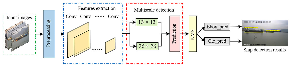
Figure 1: Diagram of the ship detection method based on semantic aggregation for video surveillance images with complex backgrounds.
Image source credit: https://github.com/jiaming-wang/SeaShips/.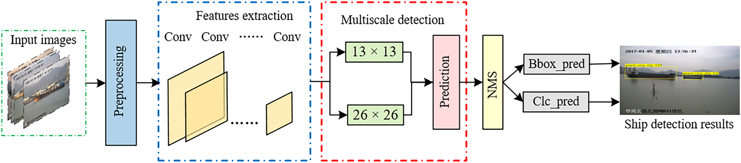
First, the input image undergoes preprocessing, which includes sizing (see ‘Multiscale input training strategy’).
Then, the Darknet-19 network is utilized for feature extraction, and both the semantic aggregation and feature fusion modules are designed to fuse deep features with rich semantic information and shallow features with rich location information, respectively. This improves the feature fusion ability.
A multiscale object detection layer is then established, utilizing feature maps with sizes of 13 × 13 pixels and 26 × 26 pixels for multiscale detection. This allows for better feature expression capabilities and enhanced detection performance, particularly for small objects such as fishing boats. The feature maps in these two layers output 1,859 (13 × 13 × 3 + 26 × 26 × 2) predicted bounding boxes.
The bounding boxes with the highest confidence scores are selected, and a comparison is made between the size of the confidence score and the threshold. A confidence score greater than the threshold indicates that the bounding boxes contain the object; otherwise, the bounding boxes do not include the object.
Finally, nonmaximum suppression (NMS) is used to select the detection results, eliminate redundant bounding boxes and obtain the position and classification results of the ship object.
YOLOv2
YOLOv2 is composed of an input layer, a feature extraction module, and a detection module. The input layer is responsible for preprocessing the image. The feature extraction module is based on the Darknet-19 network, which primarily uses 3 × 3 and 1 × 1 convolution kernels. A convolution kernel of size 1 × 1 acts as a compression tool and increases the model depth by being placed between the 3 × 3 convolution kernels. The number of convolutional filters doubles after each maximum pooling layer. Batch normalization is applied after the convolutional layer to enhance the convergence speed. The leaky rectified linear unit (ReLU) (Maas, Hannun & Ng, 2013) function is used after batch normalization to address gradient disappearance. In YOLOv2, modifications are made to the Darknet-19 network. The last convolution layer with a convolution kernel of size 1 × 1 is removed, and three convolution layers with a convolution kernel of size 3 × 3, as well as two convolution layers with a convolution kernel of size 1 × 1, are added. In addition, a route layer and a reorg layer are introduced. Consequently, YOLOv2 comprises a total of 31 layers. Table 1 provides further details on YOLOv2 when the input ship image size is 416 × 416 pixels.
| No. | Layer | Filters | Kernel size/Stride | Input Size | Output Size |
|---|---|---|---|---|---|
| 0 | Conv | 32 | 3 × 3/1 | 416 × 416 × 3 | 416 × 416 × 32 |
| 1 | Max pooling | – | 2 × 2/2 | 416 × 416 × 32 | 208 × 208 × 32 |
| 2 | Conv | 64 | 3 × 3/1 | 208 × 208 × 32 | 208 × 208 × 64 |
| 3 | Max pooling | – | 2 × 2/2 | 208 × 208 × 64 | 104 × 104 × 64 |
| 4 | Conv | 128 | 3 × 3/1 | 104 × 104 × 64 | 104 × 104 × 128 |
| 5 | Conv | 64 | 1 × 1/1 | 104 × 104 × 128 | 104 × 104 × 64 |
| 6 | Conv | 128 | 3 × 3/1 | 104 × 104 × 64 | 104 × 104 × 128 |
| 7 | Max pooling | – | 2 × 2/2 | 104 × 104 × 128 | 52 × 52 × 128 |
| 8 | Conv | 256 | 3 × 3/1 | 52 × 52 × 128 | 52 × 52 × 256 |
| 9 | Conv | 128 | 1 × 1/1 | 52 × 52 × 256 | 52 × 52 × 128 |
| 10 | Conv | 256 | 3 × 3/1 | 52 × 52 × 128 | 52 × 52 × 256 |
| 11 | Max pooling | – | 2 × 2/2 | 52 × 52 × 256 | 26 × 26 × 256 |
| 12 | Conv | 512 | 3 × 3/1 | 26 × 26 × 256 | 26 × 26 × 512 |
| 13 | Conv | 256 | 1 × 1/1 | 26 × 26 × 512 | 26 × 26 × 256 |
| 14 | Conv | 512 | 3 × 3/1 | 26 × 26 × 256 | 26 × 26 × 512 |
| 15 | Conv | 256 | 1 × 1/1 | 26 × 26 × 512 | 26 × 26 × 256 |
| 16 | Conv | 512 | 3 × 3/1 | 26 × 26 × 256 | 26 × 26 × 512 |
| 17 | Max pooling | – | 2 × 2/2 | 26 × 26 × 512 | 13 × 13 × 512 |
| 18 | Conv | 1,024 | 3 × 3/1 | 13 × 13 × 512 | 13 × 13 × 1,024 |
| 19 | Conv | 512 | 1 × 1/1 | 13 × 13 × 1,024 | 13 × 13 × 512 |
| 20 | Conv | 1,024 | 3 × 3/1 | 13 × 13 × 512 | 13 × 13 × 1,024 |
| 21 | Conv | 512 | 1 × 1/1 | 13 × 13 × 1,024 | 13 × 13 × 512 |
| 22 | Conv | 1,024 | 3 × 3/1 | 13 × 13 × 512 | 13 × 13 × 1,024 |
| 23 | Conv | 1,024 | 3 × 3/1 | 13 × 13 × 1,024 | 13 × 13 × 1,024 |
| 24 | Conv | 1,024 | 3 × 3/1 | 13 × 13 × 1,024 | 13 × 13 × 1,024 |
| 25 | Route 16 | – | – | – | 26 × 26 × 512 |
| 26 | Conv | 64 | 1 × 1/1 | 26 × 26 × 512 | 26 × 26 × 64 |
| 27 | Reorg | – | /2 | 26 × 26 × 64 | 13 × 13 × 256 |
| 28 | Route 27 24 | – | – | – | 13 × 13 × 1,280 |
| 29 | Conv | 1,024 | 3 × 3/1 | 13 × 13 × 1,280 | 13 × 13 × 1,024 |
| 30 | Conv | 55 | 1 × 1/1 | 13 × 13 × 1,024 | 13 × 13 × 55 |
| 31 | Detection |
According to Table 1, we observe that the 25th layer functions as a route layer, connecting the output feature map of the 16th layer directly to the front of the 26th layer. The 26th layer is a convolution layer that utilizes 64 convolution kernels with a size of 1 × 1. The 27th layer is a reorg layer, similar to the ResNet network shortcut, that transforms the output feature map of 26 × 26 × 64 into an output feature map of 13 × 13 × 256 to leverage the fine-grained features (i.e., features that can identify and classify local details in an image). The 28th layer (route layer) concatenates the outputs of the 24th and 27th layers to obtain a 13 × 13 × 1,280 feature map. Finally, a convolutional layer with a 3 × 3 convolutional kernel is employed for cross-channel information fusion, reducing the channels of the feature map to 1,024 and obtaining a feature map of 13 × 13 × 1,024. The 30th layer uses 55 convolutional kernels with a size of 1 × 1. Following this operation, a 13 × 13 × 55 feature map is generated, and the classification result and the width and height of the anchor box are obtained through processing this feature map.
We divide the input ship image into 13 × 13 grid cells. Each grid cell predicts multiple bounding boxes and their confidence scores. The bounding box contains five predicted values: . The represents the center point coordinates of the bounding box relative to the grid cell. The represents the width and height of the bounding box. The confidence score (Redmon et al., 2016) is defined in Eq. (1).
(1) where represents the probability that the object may appear in the box, and represents the ratio between the intersection and union of the predicted bounding box and the ground truth box. If a ship object exists in the grid cell, , the confidence score equals the (refer to using the DIoU to optimize the loss function). Otherwise, , and the confidence score is zero. 55 in the feature map of 13 × 13 × 55 refers to 5 × (6 + 5), the first five represents the number of bounding boxes per pixel grid, and the six in parentheses represents the ship categories in the SeaShips dataset (i.e., ship detection dataset). The five in parentheses represents the four coordinate values (i.e., center point coordinates, height, and width) and confidence scores for each bounding box.
Proposed ship detection method
Anchor box clustering based on the K-means method
The anchor mechanism used in Faster R-CNN is also employed in YOLOv2. Anchor boxes are a group of initial boxes with fixed sizes and aspect ratios. The selection of initial anchor boxes, whether they align with the characteristics of the detection objects or not, directly impacts the detection performance. In Faster R-CNN, the anchor boxes are manually set, which introduces personal errors. In YOLOv2, the K-means clustering method (Si et al., 2023) is used to perform clustering calculations on the ground truth boxes of the PASCAL VOC2007 dataset (Everingham et al., 2010) to obtain the optimal width, height, and number of initial anchor boxes. It should be noted that when using the Euclidean distance as a metric, larger bounding boxes may result in larger errors than smaller bounding boxes. However, in practice, we aim to obtain a high IoU value from the prior anchor box, which is not dependent on the size of the prior anchor box. Therefore, the distance metric is defined in Eq. (2).
(2) where box indicates the ground truth box of the ship object, and centroid indicates the central anchor box of the cluster. In this study, the average IoU is used as the measurement for clustering. The average IoU is the maximum average value of the IoU between the ground truth boxes and the central anchor box. The objective function for the average IoU is expressed in Eq. (3).
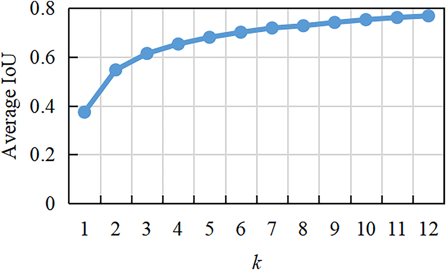
(3) where q and k depict the total number of objects and clusters, respectively, and denotes the number of samples of the th cluster center. Since the size and number of anchor boxes obtained by clustering on the PASCAL VOC2007 dataset are not suitable for the ship detection dataset, the anchor boxes of the ship detection dataset are reanalyzed by clustering, and the average IoU curve with different clustering numbers is obtained, as shown in Fig. 2. This shows that as k increases, the average IoU changes increasingly slowly. When , the average IoU increases faster. When , the average IoU becomes stable. With increasing k, the risk of model overfitting also increases. Considering the recall and complexity of the detection model, is adopted in this study. On the one hand, it can accelerate the convergence of the proposed method in the training phase, and on the other hand, it can reduce the error caused by the anchor boxes. When k is equal to five, the width and height of the initial anchor boxes are (0.982, 0.457), (2.085, 0.831), (3.683, 1.396), (6.371, 1.998), and (8.849, 3.298). The width–height ratios of the anchor boxes are (2.15, 2.51, 2.64, 2.68, 3.19). The shape of the anchor boxes is mostly short and wide, which accords with the narrow and long characteristics of the ship object in the dataset.
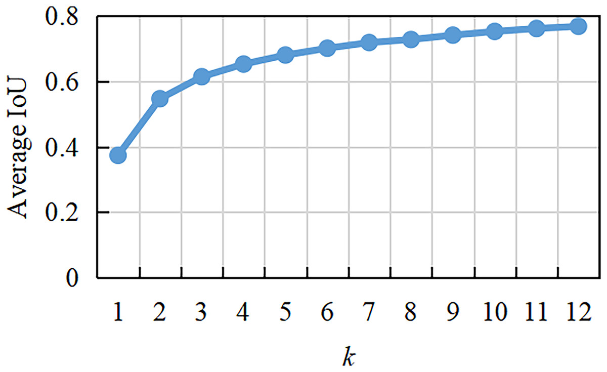
Figure 2: Average IoU at different clustering numbers.
Semantic aggregation module
The CNN extracts deep features that contain rich semantic information, giving it an advantage in predicting large objects. On the other hand, the CNN also extracts shallow features that have less semantic information but contain richer location information, which is advantageous for predicting small objects. In YOLOv2, the shallow high-resolution features undergo deformation using the reorg layer to better capture detailed information, and then they are fused with the deep low-resolution features to effectively detect objects using features from different layers, as depicted in Fig. 3A. However, YOLOv2 overlooks the incorporation of deep features with rich semantic information into shallow features, and it utilizes only a single-scale object detection layer, resulting in poor detection performance for small objects such as fishing boats. Therefore, in this article, we propose the semantic aggregation module, as shown in Fig. 3B, to enhance YOLOv2. By integrating deep features with shallow features, the model’s classification and positioning capabilities for ship objects are improved. It is worth noting that the notation “2 × upsampling” represents 2x upsampling. The specific procedure involves convolving the deep features with a 1 × 1 convolution operation and performing a 2x upsampling operation, which are then fused with the shallow features. In line with the correlation between feature maps, ship objects of various scales are detected from the fused features through lateral connections. To facilitate fusion, a 1 × 1 convolution operation is employed to adjust the channel dimension to a fixed number, and 2x upsampling is used to ensure consistent spatial resolution between deep and shallow features. In the enhanced YOLOv2 model, the semantic aggregation module is added to the 24th and 16th layers, as stated in Table 1.
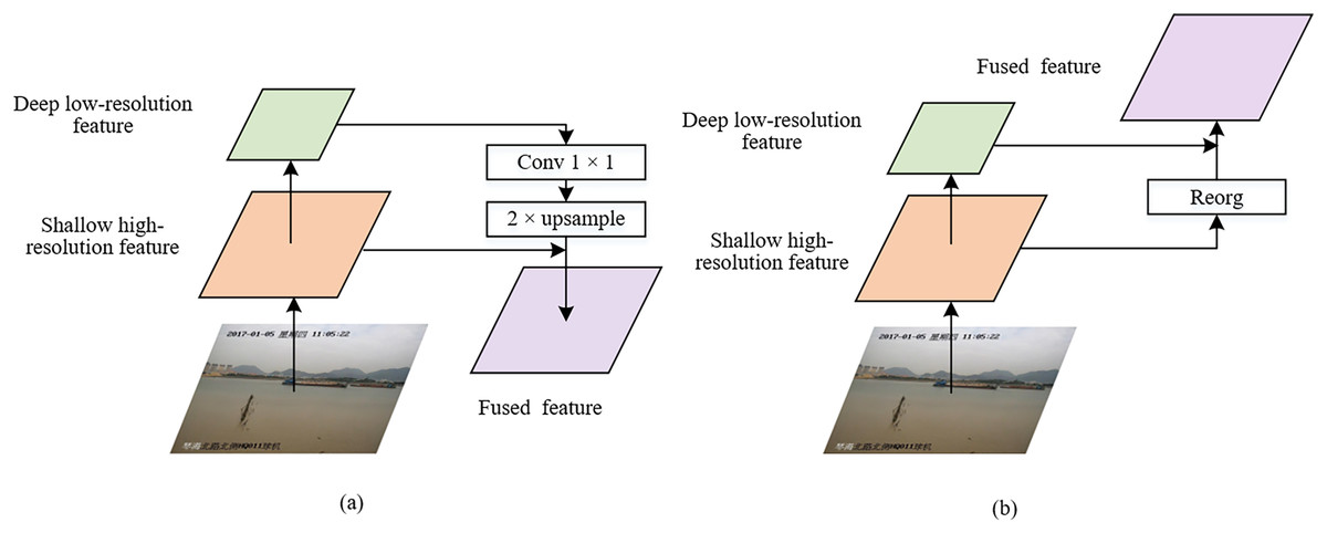
Figure 3: The feature fusion module and semantic aggregation module.
Image taken from https://github.com/jiaming-wang/SeaShips/.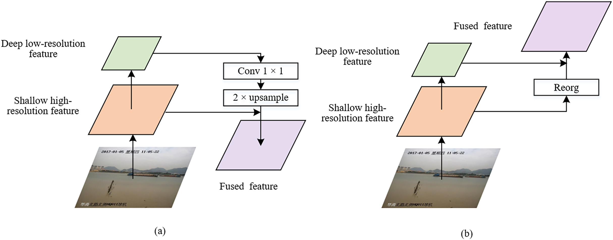
Multiscale ship detection layer
The YOLOv2 detection network utilizes only a 13 × 13 object detection layer to predict class and location details. However, this limitation restricts the perception scope, making it prone to missing or misidentifying relatively small objects or objects with a small proportion of pixels in the image due to long-range shooting. To address this, we propose the addition of a 26 × 26 object detection layer, which, in conjunction with the 13 × 13 object detection layer, maximizes the utilization of multiscale features, leading to improved ship detection across various scales. To fully integrate deep semantic features with shallow fine-grained features that are abundant in location information and enhance the detection performance for small objects, we leverage the semantic aggregation module and feature fusion module of YOLOv2 to establish a 26 × 26 object detection layer.
Figure 4 presents the multiscale ship detection layer of the enhanced ship detection model used in this study. The process for establishing the 26 × 26 object detection layer is as follows: First, the output feature map in the 10th layer (see Table 1) is transformed into a 26 × 26 × 1,024 feature map using the reorg layer. Next, the 13 × 13 × 1,024 feature map from the 24th layer undergoes a 1 × 1 convolution (with 512 convolutional kernels) and 2x upsampling via the semantic aggregation module to generate a 26 × 26 × 512 feature map. These two 26 × 26 feature maps, along with the 26 × 26 × 512 feature maps obtained from the 16th layer, are fused to create a fusion feature map of size 26 × 26 × 2,048. Finally, the fusion feature map is subject to convolution (Convs in Fig. 4 implies the initial use of 3 × 3 convolution for cross-channel information fusion, followed by 1 × 1 convolution for dimension reduction of the feature map). The feature map with reduced dimensions is then utilized to predict the objects. Furthermore, the feature map of size 52 × 52 includes rich fine-grained features and important location information of small-size objects, allowing for enhanced detection precision of small ships.
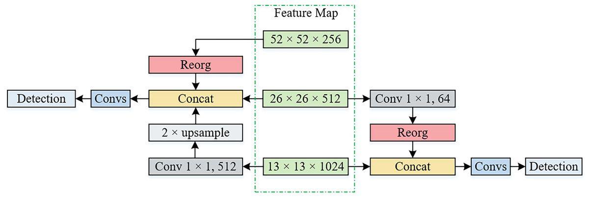
Figure 4: Multiscale ship detection layer.
The process for establishing the 13 × 13 object detection layer is as follows: The output feature map from the 16th layer (see Table 1) is subjected to a 1 × 1 convolution operation to acquire a feature map of size 26 × 26 × 64. This is subsequently reshaped into a 13 × 13 × 256 feature map using the reorg layer to leverage the fine-grained features of the model. Next, the output feature map from the 27th layer and the output feature map from the 24th layer are fused to obtain a feature map of size 13 × 13 × 1,280. Finally, cross-channel information fusion is performed using a 3 × 3 convolutional layer, followed by channel reduction through a 1 × 1 convolutional operation. The resulting feature map with reduced dimensions is employed for object prediction.
Due to the inherent characteristics of the feature maps, the feature map of size 26 × 26 employs two smaller anchor boxes ((0.982, 0.457), (2.085, 0.831)) and six categories, while the feature map of size 13 × 13 utilizes three larger anchor boxes ((3.683, 1.396), (6.371, 1.998), (8.849, 3.298)) and covers six categories.
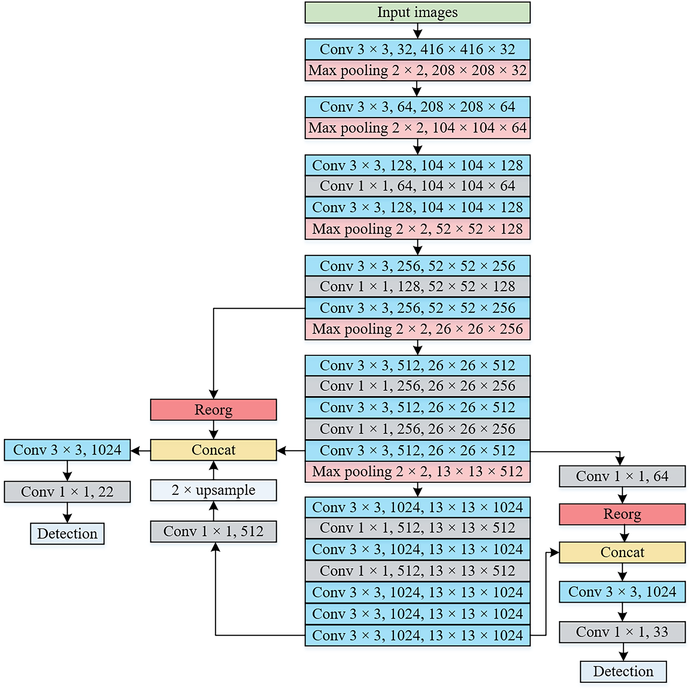
Therefore, the network architecture of the proposed method is illustrated in Fig. 5. The input image is resized to a dimension of 416 × 416 pixels. Notably, the feature extraction network includes the initial 18 convolutional layers along with two additional convolutional layers consisting of 1,024 convolution kernels measuring 3 × 3 in YOLOv2. The detection network is composed of two parts, specifically, the object detection layers that utilize 13 × 13 and 26 × 26 feature maps. In our proposed network architecture, since there are only convolution layers and pooling layers, the input image size can be dynamically adjusted. For instance, when the input image is resized to 480 × 480 pixels, the 13 × 13 and 26 × 26 feature maps are transformed to 15 × 15 and 30 × 30, respectively. In Fig. 5, the notation “Conv 3 × 3, 32, 416 × 416 × 32” represents the presence of 32 convolution kernels measuring 3 × 3, resulting in an output feature map of size 416 × 416 × 32. Similarly, “Max pooling 2 × 2, 208 × 208 × 32” denotes the utilization of a pooling kernel of size 2 × 2, leading to an output feature map of size 208 × 208 × 32. In Table 2, semantic aggregation modules are incorporated at layers 24 and 16, while the feature fusion module corresponds to layers 10 and 16, as well as layers 16 and 24.
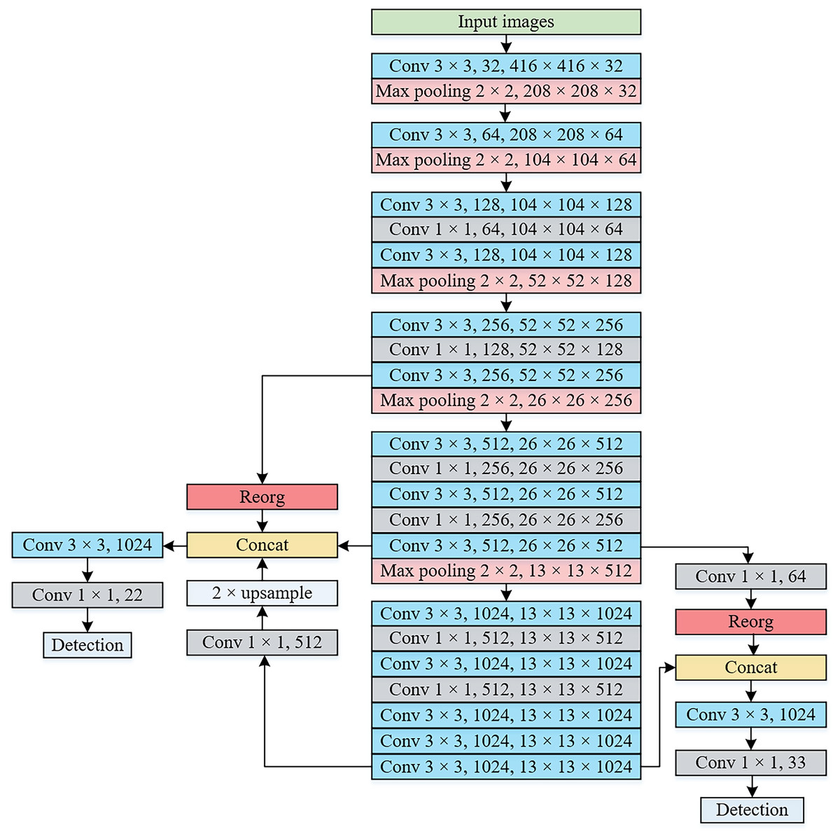
Figure 5: The network architecture of the proposed method.
| No. | Class | Train | Test |
|---|---|---|---|
| 1 | Bulk | 1,527 | 425 |
| 2 | Container | 738 | 163 |
| 3 | Fishing | 1,751 | 439 |
| 4 | General | 1,219 | 286 |
| 5 | Ore | 1,751 | 448 |
| 6 | Passenger | 382 | 92 |
| Total | 7,368 | 1,853 | |
Using the DIoU to optimize the loss function
The calculation of the YOLOv2 loss function is based on the IoU (Girshick et al., 2014), which represents the ratio between the intersection and union of the predicted bounding box and the ground truth box. It can be expressed in Eq. (4).
(4) where represents the predicted bounding box, represents the ground truth box, and denotes the area of the image region.
When there is no overlap between and , the IoU equals 0, which cannot reflect the distance between two boxes. The gradient of the loss function will be 0, and the network cannot be optimized. Moreover, if the intersection of and are the same, the IoU is the same, but their alignment modes are different. The IoU cannot accurately reflect the intersection degree of and .
To address the shortcomings of the IoU, Rezatofighi et al. (2019) proposed the generalized intersection over union (GIoU) method, which can be expressed in Eq. (5).
(5) where C represents the minimum closure region. The GIoU ranges from −1 to 1. More iterations are needed for convergence. Therefore, Zheng, Wang & Liu (2019) proposed the DIoU to directly minimize the normalized distance between the center points of and , which can be expressed in Eq. (6).
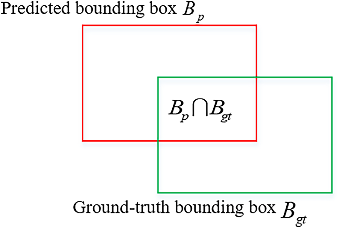
(6) where and denote the center points of and , represents the Euclidean distance, and c represents the diagonal distance of the minimum closure region containing both and . The DIoU diagram is shown in Fig. 6. The DIoU is more suitable than the GIoU for regression of object boxes. For and in the horizontal and vertical directions, the DIoU converges faster than the GIoU.
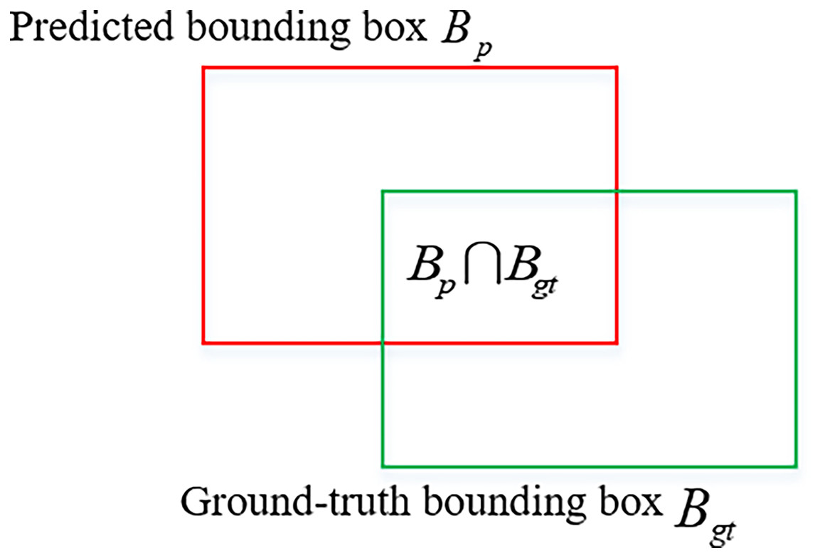
Figure 6: Distance intersection over union (DIoU).
The environment of inland waterways is complex and diverse, leading to challenges in ship detection due to crowded river conditions. To enhance ship detection effectiveness, the proposed method incorporates a loss function designed using the DIoU. The expression of the loss function is shown in Eq. (7).
(7) where denotes the confidence error of the background, represents the coordinate error of the anchor box and prediction bounding box, and represents the sum of the coordinate errors, confidence errors and classification errors of the prediction bounding boxes matched with each ground truth box. W and H are the width and height of the feature map, respectively. A is the number of anchor boxes corresponding to each grid. In Eq. (7), represent the row and column of the current target center and the category to which the current target belongs, respectively, indicates that there are no objects in the current grid, represents the weight coefficient of no object, represents the weight coefficient of the anchor box, indicates the anchor box coordinates of class k, and represents the maximum DIoU between and . When the DIoU is less than the set threshold, it is marked as the background. indicates the DIoU of and , indicates that an object exists in the anchor box, denotes the weight coefficient of the coordinate error, represents the coordinates of , denotes the coordinates of of class k, and represents the weight coefficient of the object, and depicts the IoU between and . In Eq. (7), is the weight coefficient of the category, m indicates the category of the current object, denotes the total number of categories, represents the true category of the object, and represents the category of the predicted bounding box object.
Multiscale input training strategy
To enhance the robustness of the proposed method, a multiscale input training strategy is adopted. This strategy allows for dynamic adjustment of the input image size. Since the total downsampling step size is 32, input image sizes that are multiples of 32 are selected. The minimum input image size is 320 × 320 pixels, while the maximum is 608 × 608 pixels. During the training phase, after every 10 batches, the input image size is randomly selected from {320, 352, 384, 416, 448, 480, 512, 544, 576, 608}. The corresponding final detection output feature map has a size {10, 11, 12, 13, 14, 15, 16, 17, 18, 19}. For the same training model, test set images of different sizes can be evaluated. According to the reference (Redmon & Farhadi, 2017), the object detection precision increases with increasing test set image size, but the detection speed decreases. Therefore, in this study, the input image size for the test set is set to 480 × 480 pixels, considering both the detection precision and speed. Data enhancement methods such as hue adjustment, random flipping, and exposure variation were used during training to improve the generalization ability of the model.
Results, anaysis and discussion
Ship detection dataset
The ship detection dataset utilized in this study is a subset of the publicly available SeaShips dataset (Shao et al., 2018), which consists of 7,000 images with dimensions of 1,920 × 1,080 pixels. These images were obtained from video clips captured by 156 cameras within a video surveillance system along the Pearl River in Hengqin New District, Zhuhai, China. The dataset includes diverse imaging scenarios, including variations in backgrounds, lighting, scales, and viewing angles. It is organized into six categories, namely, bulk cargo carrier, container ship, fishing boat, general cargo ship, ore carrier, and passenger ship. Figure 7 depicts visual examples of each category. For training purposes, a random selection of 5,600 samples was made, leaving 1,400 samples for testing. This resulted in a training-to-test set ratio of 4:1. The distributions of training and test samples across ship categories are presented in Table 2.
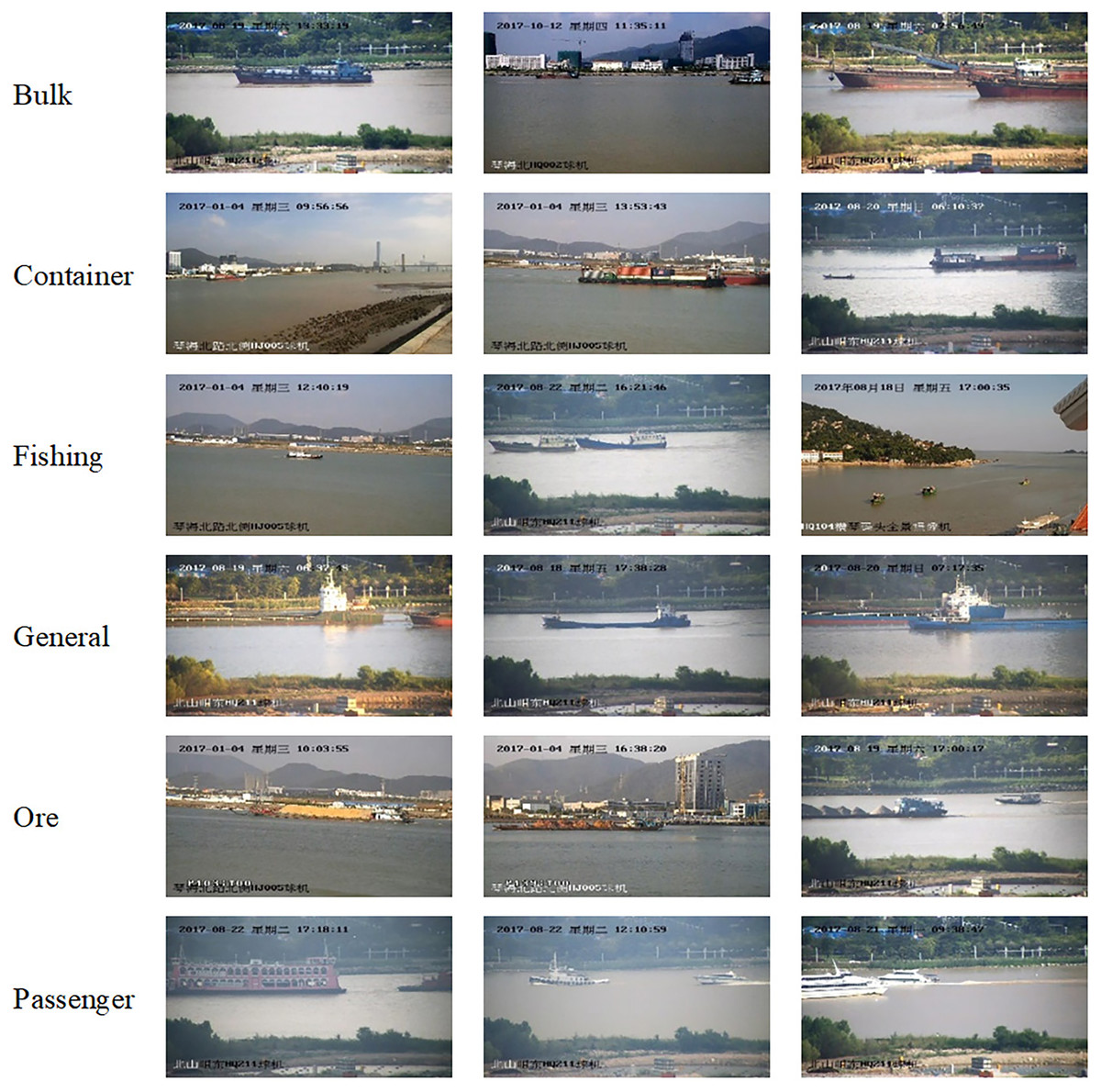
Figure 7: Visual samples of each category of the SeaShips dataset.
Image source credit: https://github.com/jiaming-wang/SeaShips/.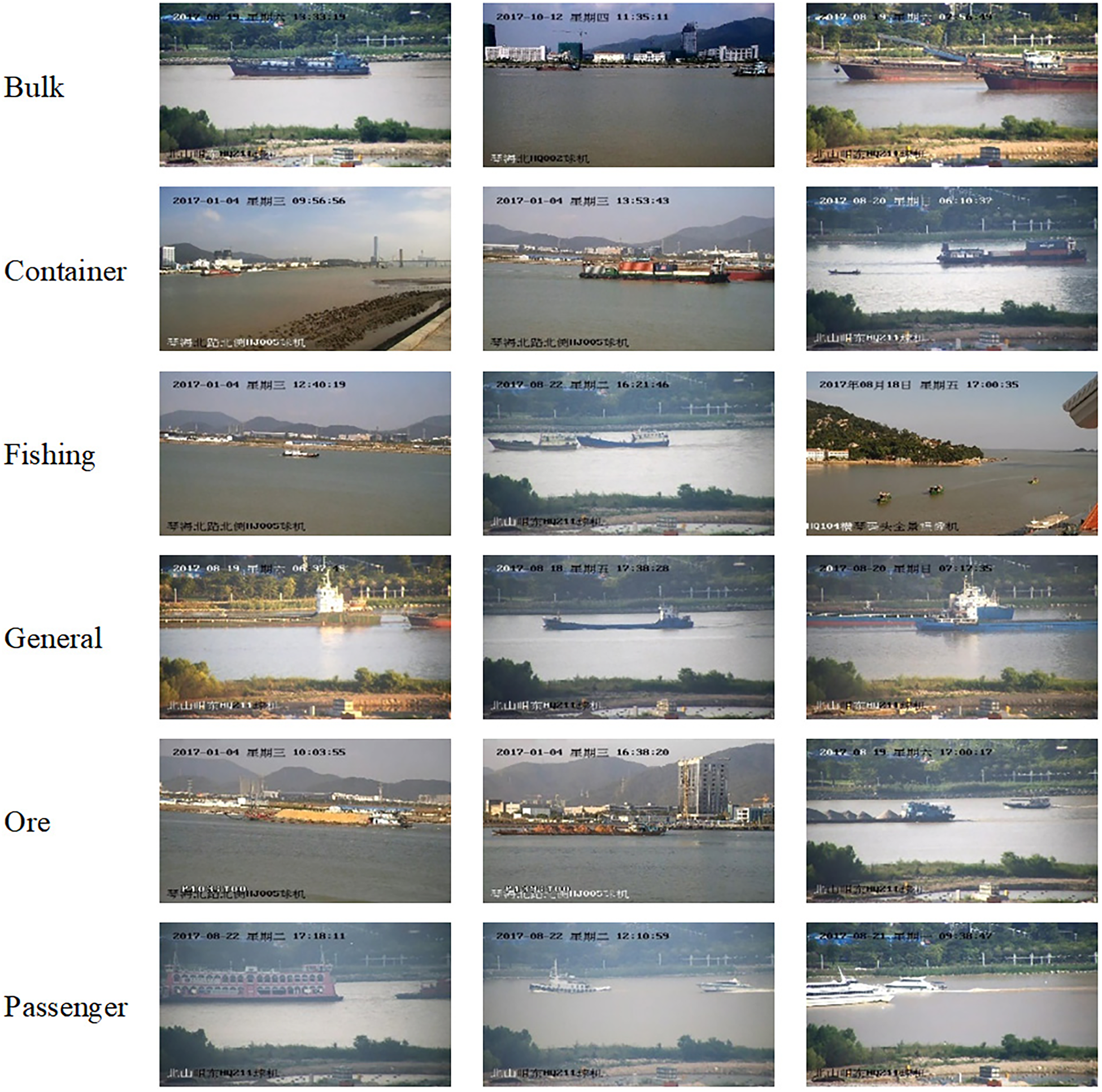
To further assess the performance of the proposed ship detection method, a second experimental dataset, named the Seaships_enlarge dataset, was used. This dataset was created by capturing video clips of ships navigating through the Wuhan section of the Yangtze River, specifically the Zhuozhou Yangtze River Bridge, the Wuhan Yangtze River Bridge, and the Second Wuhan Yangtze River Bridge. From these video clips, one frame image was extracted every 50 frames, resulting in a total of 983 ship images after removing highly similar images. Due to the limited number of ship images available, validating the algorithm’s detection performance alone proved difficult. Consequently, these images were added to the existing Seaships dataset, resulting in an expanded dataset called Seaships_enlarge. The training set of Seaships_enlarge comprises 6,386 samples, while the remaining 1,597 samples serve as the test images. Table 3 displays the distribution of training and test samples within the Seaships_enlarge dataset. To facilitate comparative experiments, 1,436 images from the Seaships dataset, belonging to the test set, were chosen as the new test set and are listed under the “test_new” column in Table 3. To annotate the ship’s transverse and longitudinal coordinates, length, and width within the 983 ship images, the LabelImg (Tzutalin, 2018) annotation tool was utilized. The resulting annotations were generated in XML format, adhering to the annotation format of the PASCAL VOC2007 dataset.
| No. | Class | Train | Test | Test_new |
|---|---|---|---|---|
| 1 | Bulk | 1,780 | 401 | 362 |
| 2 | Container | 854 | 227 | 201 |
| 3 | Fishing | 1,719 | 471 | 471 |
| 4 | General | 1,643 | 444 | 340 |
| 5 | Ore | 1,897 | 442 | 418 |
| 6 | Passenger | 762 | 169 | 100 |
| Total | 8,655 | 2,154 | 1,892 | |
Evaluation metrics
To evaluate the performance of the proposed method, the following metrics were employed: AP, mean average precision (mAP), frames per second (FPS), model size and giga floating-point operations per second (GFLOPs).
The AP (Powers, 2020) refers to the area of the graph enclosed by a precision-recall curve (i.e., P-R curve), with precision represented on the vertical axis and recall on the horizontal axis. The expression for AP is shown in Eq. (8).
(8)
Precision (Powers, 2020) reflects the accuracy of the detector in predicting positive samples, while recall (Powers, 2020) reflects the detector’s ability to detect positive samples. They are calculated in Eqs. (9) and (10).
(9)
(10) where TP, FP and FN denote the number of samples correctly detected, samples incorrectly detected, and samples not detected, respectively, but in fact, there are ship objects in the image.
The mAP (Everingham et al., 2010) represents the mean AP and combines the precision and recall to evaluate the method’s performance. A higher mAP indicates better detection effectiveness. It is expressed in Eq. (11).
(11) where n denotes the number of ship classes, [email protected] is calculated when the IoU threshold is 0.5.
The FPS can evaluate the detection speed of the method. It indicates the number of images processed per second. The larger the FPS is, the faster the detection speed.
The model size can measure the number of parameters. The GFLOPs reflects the calculation cost and running speed of the model.
Experimental configuration and parameters
The experiment was conducted on a server with an Intel® Core™ i9-7980XE CPU, 32 GB of RAM, an NVIDIA TITAN Xp Pascal graphics card, and a Windows 10 operating system. The software environment used was Python 3.7 and the PyTorch deep learning framework.
The parameter settings are as follows: the input images are 416 × 416 pixels, the batch size is 64, the initial learning rate is set to 0.0001, and the learning decay step boundaries are “400, 700, 900, 1,000, and 15,000,” with corresponding learning rates of 0.0001, 0.0005, 0.0005, 0.001, and 0.0001, respectively. The stochastic gradient descent (SGD) method is used during the training phase. The maximum number of iterations is set at 17,500, the momentum parameter is 0.9, and the weight decay is 0.0005. The probability of random flipping is 0.5, the saturation and exposure change size is 1 to 1.5 times, and the hue change range is −0.1 to 0.1. is 1, is 1, is 5, is 1, is 0, and the threshold is 0.6. The confidence threshold is 0.1, and the DIoU threshold is set as 0.5.
Detection results and analysis
Performance on the SeaShips dataset
To assess the performance of the proposed method, it is compared to Faster R-CNN (Ren et al., 2017), SSD (Liu et al., 2016), YOLOv2 (Redmon & Farhadi, 2017), method (Shao et al., 2020), method (Liu et al., 2021), FCOS (Law & Heng, 2018), method (Lin et al., 2020), YOLOv3-tiny (Wang & Wang, 2023), YOLOv4 (Wang & Wang, 2023), YOLOv5s (Wang & Wang, 2023) and YOLOv8s (Luo, Li & He, 2024) on the SeaShips dataset under the same experimental conditions. VGG16 is used as the feature extraction network for Faster R-CNN and SSD.
The detection performance is evaluated from both quantitative and qualitative perspectives.
Quantitative analysis
Table 4 presents a comprehensive comparison of various methods for the SeaShips dataset, including [email protected], AP for each ship type, and FPS. Notably, the Faster R-CNN and method (Lin et al., 2020) achieved the higher [email protected], reaching 90.33% and 89.90%, respectively. However, their FPS is only 6 and 5, which is lower than those of the other methods listed in Table 4. Although SSD and FCOS have shown some improvement in detection speed, they are unable to achieve real-time detection (which is typically considered to be at 24 FPS in object detection). Similarly, although YOLOv2 boasts a detection speed of 34 FPS, its [email protected] is 5.18% and 1.83% lower than those of Faster R-CNN and SSD, respectively. Additionally, in regard to the fishing boat category, the APs of YOLOv2 are 14.69% and 8.89% lower than those of Faster R-CNN and SSD, respectively. The reason for this disparity lies in the fact that the fishing boat is classified and positioned on the feature map after 32 rounds of subsampling, even though it only occupies a small portion of the original 1,920 × 1,080 pixel image (approximately 70 × 130 pixels). Consequently, YOLOv2 often fails to capture vital information pertaining to small ships, resulting in poor detection performance for these vessels. In contrast, our proposed method increases the [email protected] by 2.32% and 4.15% compared to SSD and YOLOv2, respectively. Notably, the proposed method shows notable improvements in AP for bulk ships and ore carriers, as these ships differ significantly from others due to their specific cargo—bulk goods and ore, respectively. Furthermore, the [email protected] of our proposed method also surpasses that of method (Shao et al., 2020), method (Liu et al., 2021), YOLOv3-tiny, YOLOv4 and YOLOv5s. In particular, the AP for fishing boats in our proposed method exhibited the most substantial increase, increasing by 10.98% compared to that in method (Shao et al., 2020). This enhanced performance can be attributed to two key factors. First, the addition of a semantic aggregation module improves the method’s ability to classify and locate ship objects. Second, a large-scale object detection layer is incorporated, enhancing the detection functionality for small ships. Moreover, our proposed method employs a loss function based on the DIoU, further enhancing the overall detection effectiveness. Further, by comparing AP, it can be seen that the proposed method can obtain good detection performance for different types of ships. Although the adoption of a multiscale object detection layer and the increase in parameters in our proposed method reduce the detection speed compared to YOLOv2, YOLOv3-tiny and YOLOv5s, it still maintains a speed that is 1.47 times faster than YOLOv4 and 2.33 times faster than FCOS. Therefore, the proposed method adequately meets the requirements for real-time detection. Compared with the YOLOv8s, [email protected] is slightly reduced in the proposed method, but the semantic aggregation module and multi-scale object detection layer are used in the proposed method to improve ship detection performance. Compared with the other existing ship detection techniques, the proposed method can effectively improve the precision of ship detection and ensure the detection efficiency. However, YOLOv8s has high requirements on hardware, requires a large amount of GPU resources and high memory of the graphics card, which increases the use cost and maintenance difficulty.
| Method | AP | [email protected] (%) | FPS | |||||
|---|---|---|---|---|---|---|---|---|
| Bulk | Container | Fishing | General | Ore | Passenger | |||
| Faster R-CNN (Ren et al., 2017) | 0.903 | 0.909 | 0.888 | 0.907 | 0.894 | 0.906 | 90.10 | 6 |
| SSD (Liu et al., 2016) | 0.877 | 0.909 | 0.843 | 0.889 | 0.882 | 0.819 | 86.98 | 11 |
| YOLOv2 (Redmon & Farhadi, 2017) | 0.867 | 0.909 | 0.768 | 0.868 | 0.898 | 0.780 | 85.15 | 34 |
| Method (Shao et al., 2020) | 0.876 | 0.903 | 0.783 | 0.917 | 0.881 | 0.886 | 87.40 | 49 |
| Method (Liu et al., 2021) | 0.852 | 0.911 | 0.895 | 0.880 | 0.906 | 0.821 | 87.74 | 30 |
| Method (Lin et al., 2020) | 0.886 | 0.909 | 0.899 | 0.901 | 0.900 | 0.901 | 89.90 | 5 |
| FCOS (Law & Heng, 2018) | 0.901 | 0.909 | 0.904 | 0.906 | 0.900 | 0.903 | 90.40 | 12 |
| YOLOv3-tiny (Wang & Wang, 2023) | – | – | – | – | – | – | 78.39 | 48 |
| YOLOv4 (Wang & Wang, 2023) | – | – | – | – | – | – | 87.45 | 19 |
| YOLOv5s (Wang & Wang, 2023) | – | – | – | – | – | – | 85.56 | 97 |
| YOLOv8s (Luo, Li & He, 2024) | – | – | – | – | – | – | 91.34 | 102 |
| Proposed method | 0.892 | 0.909 | 0.869 | 0.899 | 0.902 | 0.886 | 89.30 | 28 |
Table 5 shows the model size and GFLOPs of different methods for the SeaShips dataset. It can be seen that the GFLOPs of proposed method is smaller than that of Faster R-CNN, SSD, method (Lin et al., 2020), FCOS and YOLOv4. And the GFLOPs of the proposed method only increases by 3.39 and 4.34 compared to that in YOLOv2 and YOLOv8s, respectively. The model size of the proposed method is smaller than that of the method (Lin et al., 2020) and YOLOv4, and slightly larger than that of YOLOv2. In general, the proposed method meets the requirement of real-time detection, and it achieves better detection performance.
| Method | GFLOPs | Model size (MB) |
|---|---|---|
| Faster R-CNN (Ren et al., 2017) | 272.46 | 108 |
| SSD (Liu et al., 2016) | 137.30 | 93.10 |
| YOLOv2 (Redmon & Farhadi, 2017) | 29.65 | 92.53 |
| Method (Lin et al., 2020) | 81.90 | 144.52 |
| FCOS (Law & Heng, 2018) | 126.38 | 41.12 |
| YOLOv3-tiny (Wang & Wang, 2023) | 18.90 | 24.40 |
| YOLOv4 (Wang & Wang, 2023) | 60.50 | 244 |
| YOLOv5s (Wang & Wang, 2023) | 16.41 | 14.20 |
| YOLOv8s (Luo, Li & He, 2024) | 28.70 | 43.70 |
| Proposed method | 33.04 | 129.39 |
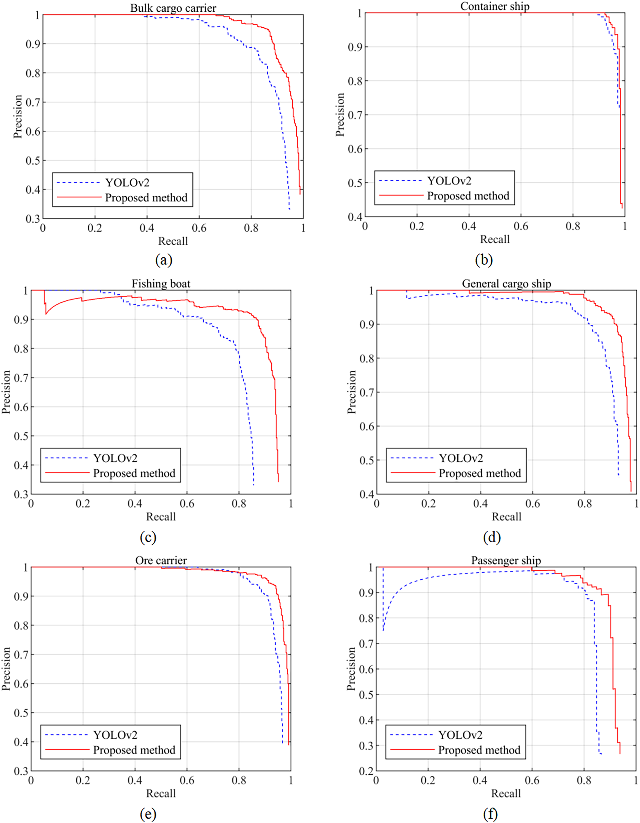
Figure 8 presents a comparison of the precision‒recall curves between the proposed method and YOLOv2 for six different ship types. It is evident from the graph that the proposed method achieves a higher recall for all six ship types while maintaining the same precision. Additionally, the area enclosed by the solid curve and coordinate axis is also larger for the proposed method, indicating its superior detection performance compared to YOLOv2. Furthermore, as depicted in Fig. 8B, the proposed method exhibits a relatively smaller improvement in the AP for container ships compared to YOLOv2. Consequently, the precision–recall curve appears to be closer for this specific ship type. However, overall, the [email protected] of the proposed method surpasses that of YOLOv2.
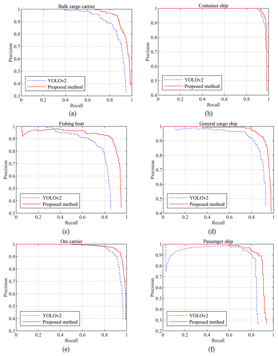
Figure 8: (A–F) Precision‒recall curves of the two models for six ship types.
Qualitative analysis
According to the qualitative analysis illustrated in Fig. 9, the visual detection results of both the YOLOv2 method and the proposed method on selected ship samples from the SeaShips dataset are presented. Figures 9A, 9C, 9E, 9G, and 9I demonstrate the visual detection results of YOLOv2, while Figs. 9B, 9D, 9F, 9H, and 9J show the visual detection results of the proposed method. Comparing Figs. 9A, 9B, 9C, and 9D, it can be observed that the YOLOv2 method misidentifies a general cargo ship as a passenger ship when the ship and background exhibit similarities. Conversely, the proposed method avoids such misidentification by differentiating between similar backgrounds and ships. Contrasting Figs. 9E and 9F, it becomes apparent that when ship objects are partially obscured, YOLOv2 generates two detection results with significant overlap for the same object, with the positioning anchor being considerably larger than the ship object itself. On the other hand, the proposed method delivers more accurate ship positioning and exhibits improved detection effectiveness. Examining Figs. 9G and 9H, it is evident that YOLOv2 experiences positioning errors when detecting remote small fishing boats. Conversely, the proposed method excels in detecting such small fishing boats, resulting in enhanced confidence scores. In Figs. 9I and 9J, YOLOv2 erroneously detects a remote small fishing boat as a passenger ship. In contrast, the proposed method accurately detects remote small fishing boats, avoiding misidentification. Overall, the proposed method demonstrates its ability to detect ship objects more effectively, accurately position them, and prevent similar background misidentifications when there are occlusions between ship objects and small ships at a distance. However, as observed in Fig. 9J, the proposed method still exhibits some deviations in the positioning anchor box for smaller fishing boats. Future research will focus on further improving the detection performance for small-size ships.
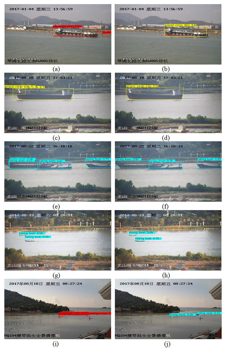
Figure 9: Visual detection results of partial ship samples in the SeaShips test set.
(A), (C), (E), (G), and (I) are the detection results of the YOLOv2 method; (B), (D), (F), (H), and (J) are the detection results of the proposed method. Image source credit: https://github.com/jiaming-wang/SeaShips/.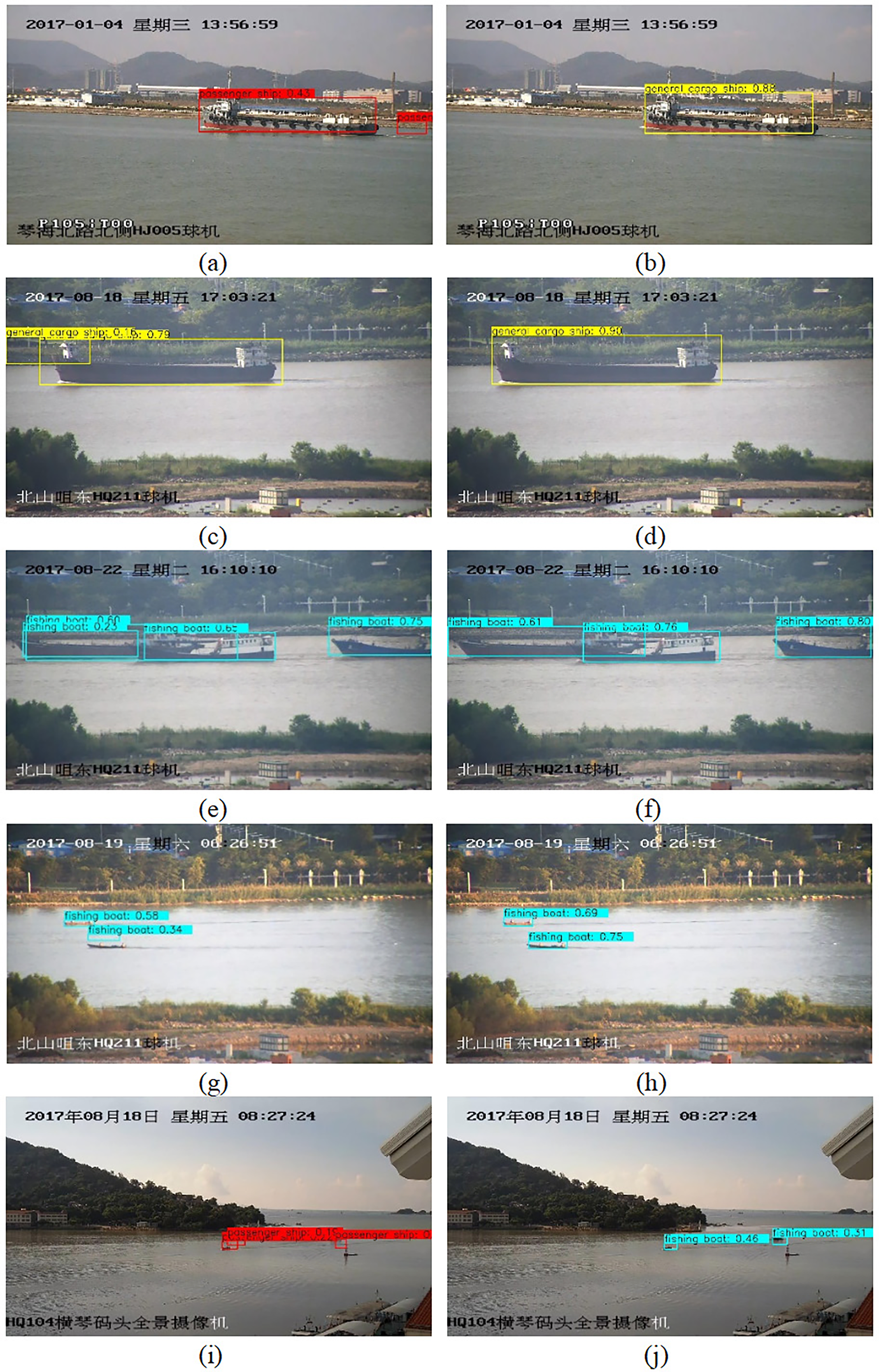
Analysis of influencing factors
To analyze the influence of each improved module on the detection performance, experiments were conducted on the SeaShips dataset. The results are presented in Table 6. In the case of using the IoU loss function, compared with YOLOv2, the semantic aggregation module and multiscale object detection layer improved the localization and classification performance of ship objects, resulting in an increase in the [email protected] of 3.42%. By using the GIoU loss function, the ship detection performance improved to a certain extent, increasing the [email protected] from 88.57% to 88.76%. Furthermore, by using the DIoU loss function, the [email protected] further increased from 88.76% to 89.30%. These results indicate that the use of the semantic aggregation module and multiscale object detection layer can enhance the detection effect of ship objects, while the DIoU loss function, which is more consistent with the object anchor box regression mechanism, can further improve the detection performance.
| YOLOv2 | Semantic aggregation module and multi-scale object detection layer | IoU | GIoU (Rezatofighi et al., 2019) | DIoU (Zheng, Wang & Liu, 2019) | [email protected](%) |
|---|---|---|---|---|---|
| √ | √ | 85.15 | |||
| √ | √ | √ | 88.57 | ||
| √ | √ | √ | 88.76 | ||
| √ | √ | √ | 89.30 |
Performance on the SeaShips_enlarge dataset
To further validate the detection performance, experiments were also conducted on the SeaShips_enlarge dataset.
Quantitative analysis
The results of the quantitative analysis are presented in Table 7, which lists the AP, [email protected], and FPS for the SeaShips_enlarge dataset. The [email protected] on the new test set is 89.10%, which is 0.73% higher than that on the SeaShips_enlarge dataset. The AP of each type of ship also increased to different degrees, indicating that the diversity of samples in the dataset increased after supplementing the ship images collected in the Yangtze River. As a result, the trained detection model obtained was more robust, leading to better detection performance.
| Training set | Test set | Class | [email protected] (%) | FPS | |||||
|---|---|---|---|---|---|---|---|---|---|
| Bulk | Container | Fishing | General | Ore | Passenger | ||||
| SeaShips_enlarge | SeaShips_enlarge | 0.8882 | 0.9078 | 0.8623 | 0.8759 | 0.8928 | 0.8760 | 88.38 | 28 |
| SeaShips_enlarge | New test set | 0.8930 | 0.9081 | 0.8647 | 0.8943 | 0.8974 | 0.8893 | 89.10 | 28 |
Qualitative analysis
The qualitative analysis is depicted in Fig. 10, which displays the visual detection results of partial ship samples of the proposed method on the Seaships_enlarge dataset. The proposed method can correctly detect ship objects even under small-size and strong light conditions (Figs. 10A–10D). Additionally, ship objects can also be effectively detected when the objects are dense, the background is complex, or obstructions occur (Figs. 10E–10H).
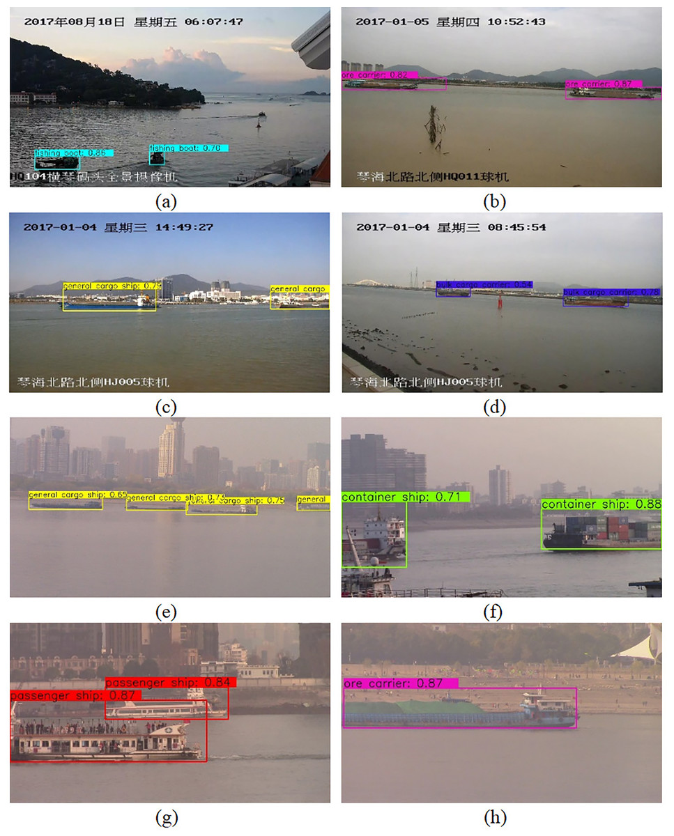
Figure 10: (A–H) Visualization examples of detection results of the proposed method for the Seaships_enlarge dataset.
Image source credit: https://github.com/jiaming-wang/SeaShips/ and https://github.com/00shannxi/983_new-ship-images.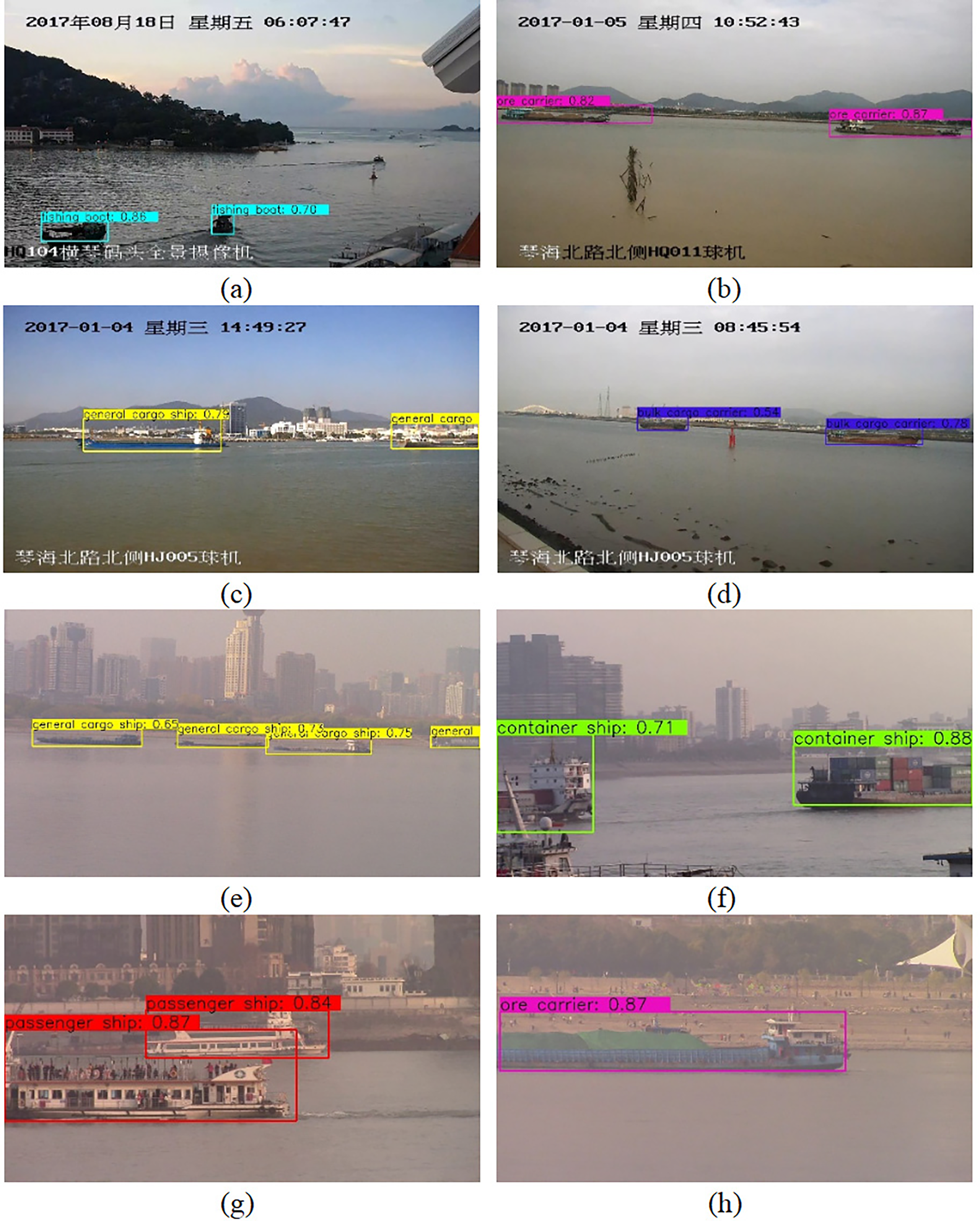
Conclusions and discussions
In this study, a ship detection method based on semantic aggregation for video surveillance images on complex backgrounds is proposed. First, suitable anchor boxes for the ship image dataset are obtained via the K-means clustering algorithm. Then, the semantic aggregation and feature fusion modules are utilized to enhance the ability to distinguish and locate ship objects. Additionally, a large-scale object detection layer is incorporated to improve the detection performance for small ships. Finally, the DIoU loss function is employed to further enhance the detection effectiveness. The experimental results demonstrate that the proposed method can enhance the [email protected] of ship objects while ensuring real-time detection compared to other methods. Specifically, the [email protected] of the SeaShips dataset and the SeaShips_enlarge dataset can reach 89.3% and 88.38%, respectively.
However, the proposed method also has some shortcomings.
(1) The multi-scale object detection layer is adopted, the number of parameters is increased, and the model is not lightweight enough. Although the detection speed of the proposed method achieves real-time detection, the FPS still lags behind that of the YOLOv3-tiny and YOLOv5s.
(2) The detection precision of the proposed method has some room for improvement.
(3) The proposed method is limited to the algorithm level and has not been deployed to the edge mobile platform.
(4) The proposed method does not consider ship detection under extreme weather conditions such as foggy weather.
(5) The semantic aggregation model has not been tested in other mainstream object detection models.
In the future research, our work mainly includes the following aspects:
(1) We will further study the use of lightweight network architecture to reduce model parameters and improve the FPS of the algorithm.
(2) Multimodal ship detection will be studied, and visible images ship detection and infrared images ship detection are fused to improve the detection performance of the algorithm.
(3) The designed model will be transplanted to the edge mobile platform for real-time applications.
(4) The image de-fogging algorithm will be studied, and the ship image after de-fogging will be detected to enhance the perception ability of the algorithm under different weather environments.
(5) The implementation of the semantic aggregation module in the latest YOLO version.