
Quantifying the effect of sentiment on information diffusion in social media
- Published
- Accepted
- Received
- Academic Editor
- Ciro Cattuto
- Subject Areas
- Data Mining and Machine Learning, Data Science, Network Science and Online Social Networks
- Keywords
- Computational social science, Social networks, Social media, Sentiment analysis, Information diffusion
- Copyright
- © 2015 Ferrara and Yang
- Licence
- This is an open access article distributed under the terms of the Creative Commons Attribution License, which permits unrestricted use, distribution, reproduction and adaptation in any medium and for any purpose provided that it is properly attributed. For attribution, the original author(s), title, publication source (PeerJ Computer Science) and either DOI or URL of the article must be cited.
- Cite this article
- 2015. Quantifying the effect of sentiment on information diffusion in social media. PeerJ Computer Science 1:e26 https://doi.org/10.7717/peerj-cs.26
Abstract
Social media has become the main vehicle of information production and consumption online. Millions of users every day log on their Facebook or Twitter accounts to get updates and news, read about their topics of interest, and become exposed to new opportunities and interactions. Although recent studies suggest that the contents users produce will affect the emotions of their readers, we still lack a rigorous understanding of the role and effects of contents sentiment on the dynamics of information diffusion. This work aims at quantifying the effect of sentiment on information diffusion, to understand: (i) whether positive conversations spread faster and/or broader than negative ones (or vice-versa); (ii) what kind of emotions are more typical of popular conversations on social media; and, (iii) what type of sentiment is expressed in conversations characterized by different temporal dynamics. Our findings show that, at the level of contents, negative messages spread faster than positive ones, but positive ones reach larger audiences, suggesting that people are more inclined to share and favorite positive contents, the so-called positive bias. As for the entire conversations, we highlight how different temporal dynamics exhibit different sentiment patterns: for example, positive sentiment builds up for highly-anticipated events, while unexpected events are mainly characterized by negative sentiment. Our contribution represents a step forward to understand how the emotions expressed in short texts correlate with their spreading in online social ecosystems, and may help to craft effective policies and strategies for content generation and diffusion.
Introduction
The emerging field of computational social science has been focusing on studying the characteristics of techno-social systems (Lazer et al., 2009; Vespignani, 2009; Kaplan & Haenlein, 2010; Asur & Huberman, 2010; Cheng et al., 2014) to understand the effects of technologically-mediated communication on our society (Gilbert & Karahalios, 2009; Ferrara, 2012; Tang, Lou & Kleinberg, 2012; De Meo et al., 2014; Backstrom & Kleinberg, 2014). Research on information diffusion focused on the complex dynamics that characterize social media discussions (Java et al., 2007; Huberman, Romero & Wu, 2009; Bakshy et al., 2012; Ferrara et al., 2013a) to understand their role as central fora to debate social issues (Conover et al., 2013b; Conover et al., 2013a; Varol et al., 2014), to leverage their ability to enhance situational, social, and political awareness (Sakaki, Okazaki & Matsuo, 2010; Centola, 2010; Centola, 2011; Bond et al., 2012; Ratkiewicz et al., 2011; Metaxas & Mustafaraj, 2012; Ferrara et al., 2014), or to study susceptibility to influence and social contagion (Aral, Muchnik & Sundararajan, 2009; Aral & Walker, 2012; Myers, Zhu & Leskovec, 2012; Anderson et al., 2012; Lerman & Ghosh, 2010; Ugander et al., 2012; Weng & Menczer, 2013; Weng, Menczer & Ahn, 2014). The amount of information that generated and shared through online platforms like Facebook and Twitter yields unprecedented opportunities to millions of individuals every day (Kwak et al., 2010; Gomez Rodriguez, Leskovec & Schölkopf, 2013; Ferrara et al., 2013b). Yet, how understanding of the role of the sentiment and emotions conveyed through the content produced and consumed on these platforms is shallow.
In this work we are concerned in particular with quantifying the effect of sentiment on information diffusion in social networks. Although recent studies suggest that emotions are passed via online interactions (Harris & Paradice, 2007; Mei et al., 2007; Golder & Macy, 2011; Choudhury, Counts & Gamon, 2012; Kramer, Guillory & Hancock, 2014; Ferrara & Yang, 2015; Beasley & Mason, 2015), and that many characteristics of the content may affect information diffusion (e.g., language-related features (Nagarajan, Purohit & Sheth, 2010), hashtag inclusion (Suh et al., 2010), network structure (Recuero, Araujo & Zago, 2011), user metadata (Ferrara et al., 2014)), little work has been devoted to quantifying the extent to which sentiment drives information diffusion in online social media. Some studies suggested that content conveying positive emotions could acquire more attention (Kissler et al., 2007; Bayer, Sommer & Schacht, 2012; Stieglitz & Dang-Xuan, 2013) and trigger higher levels of arousal (Berger, 2011), which can further affect feedback and reciprocity (Dang-Xuan & Stieglitz, 2012) and social sharing behavior (Berger & Milkman, 2012).
In this study, we take Twitter as scenario, and we explore the complex dynamics intertwining sentiment and information diffusion. We start by focusing on content spreading, exploring what effects sentiment has on the diffusion speed and on content popularity. We then shift our attention to entire conversations, categorizing them into different classes depending on their temporal evolution: we highlight how different types of discussion dynamics exhibit different types of sentiment evolution. Our study timely furthers our understanding of the intricate dynamics intertwining information diffusion and emotions on social media.
Materials and Methods
Sentiment analysis
Sentiment analysis was proven an effective tool to analyze social media streams, especially for predictive purposes (Pang & Lee, 2008; Bollen, Mao & Zeng, 2011; Bollen, Mao & Pepe, 2011; Le, Ferrara & Flammini, 2015). A number of sentiment analysis methods have been proposed to date to capture content sentiment, and some have been specifically designed for short, informal texts (Akkaya, Wiebe & Mihalcea, 2009; Paltoglou & Thelwall, 2010; Hutto & Gilbert, 2014). To attach a sentiment score to the tweets in our dataset, we here adopt a SentiStrength, a promising sentiment analysis algorithm that, if compared to other tools, provides several advantages: first, it is optimized to annotate short, informal texts, like tweets, that contain abbreviations, slang, and the like. SentiStrength also employs additional linguistic rules for negations, amplifications, booster words, emoticons, spelling corrections, etc. Research applications of SentiStrength to MySpace data found it particularly effective at capturing positive and negative emotions with, respectively, 60.6% and 72.8% accuracy (Thelwall et al., 2010; Thelwall, Buckley & Paltoglou, 2011; Stieglitz & Dang-Xuan, 2013).
The algorithm assigns to each tweet t a positive S+(t) and negative S−(t) sentiment score, both ranging between 1 (neutral) and 5 (strongly positive/negative). Starting from the sentiment scores, we capture the polarity of each tweet t with one single measure, the polarity score S(t), defined as the difference between positive and negative sentiment scores: (1)
The above-defined score ranges between −4 and +4. The former score indicates an extremely negative tweet, and occurs when S+(t) = 1 and S−(t) = 5. Vice-versa, the latter identifies an extremely positive tweet labeled with S+(t) = 5 and S−(t) = 1. In the case S+(t) = S−(t)—positive and negative sentiment scores for a tweet t are the same— the polarity S(t) = 0 of tweet t is considered as neutral.
We decided to focus on the polarity score (rather than the two dimensions of sentiment separately) because previous studies highlighted the fact that measuring the overall sentiment is easier and more accurate than trying to capture the intensity of sentiment—this is especially true for short texts like tweets, due to the paucity of information conveyed in up to 140 characters (Thelwall et al., 2010; Thelwall, Buckley & Paltoglou, 2011; Stieglitz & Dang-Xuan, 2013; Ferrara & Yang, 2015).
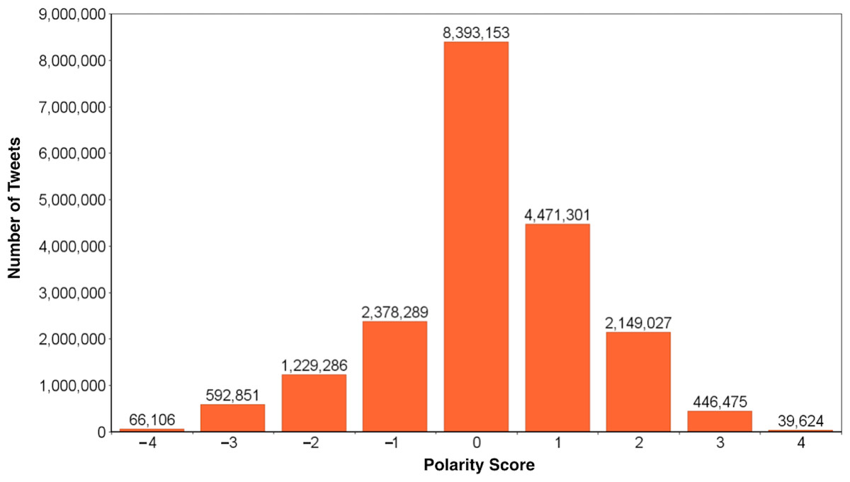
Figure 1: Distribution of polarity scores computed for our dataset.
The polarity score S is the difference between positive and negative sentiment scores as calculated by SentiStrength. The dataset (N = 19,766,112 tweets, by M = 8,130,481 different users) contains 42.46% of neutral (S = 0), 35.95% of positive (S ≥ 1), and 21.59% of negative (S ≤ − 1) tweets, respectively.
Data
The dataset adopted in this study contains a sample of all public tweets produced during September 2014. From the Twitter gardenhose (a roughly 10% sample of the social stream that we process and store at Indiana University) we extracted all tweets in English that do not contain URLs or media content (photos, videos, etc.) produced in that month. This choice is dictated by the fact that we can hardly computationally capture the sentiment or emotions conveyed by multimedia content, and processing content from external resources (such as webpages, etc.) would be computationally hard. This dataset comprises of 19,766,112 tweets (more than six times larger than the Facebook experiment (Kramer, Guillory & Hancock, 2014)) produced by 8,130,481 distinct users. All tweets are processed by SentiStrength and attached with sentiment scores (positive and negative) and with the polarity score calculated as described before. We identify three classes of tweets’ sentiment: negative (polarity score S ≤ − 1), neutral (S = 0), and positive (S ≥ 1). Negative, neutral, and positive tweets account for, respectively, 21.59%, 42.46% and 35.95% of the total. The distribution of polarity scores is captured by Fig. 1: we can see it is peaked around neutral tweets, accounting for over two-fifths of the total, while overall the distribution is slightly skewed toward positiveness. We can also observe that extreme values of positive and negative tweets are comparably represented: for example, there are slightly above 446 thousand tweets with polarity score S = + 3, and about 592 thousands with opposite polarity of S = − 3.
Results
The role of sentiment on information diffusion
Here we are concerned with studying the relation between content sentiment and information diffusion. Figure 2 shows the effect of content sentiment on the information diffusion dynamics and on content popularity. We measure three aspects of information diffusion, as function of tweets polarity scores: Fig. 2A shows the average number of retweets collected by the original posts as function of the polarity expressed therein; similarly, Fig. 2B shows the average number of times the original tweet has been favorited; Fig. 2C illustrates the speed of information diffusion, as reflected by the average number of seconds that occur between the original tweet and the first retweet. Both Figs. 2A and 2C focus only on tweets that have been retweeted at least once. Figure 2B considers only tweets that have been favorited at least once. Note that a large fraction of tweets are never retweeted (79.01% in our dataset) or favorited (87.68%): Fig. 2A is based on the 4,147,519 tweets that have been retweeted at least once (RT ≥ 1), Fig. 2B reports on the 2,434,523 tweets that have favorited at least once, and Fig. 2C is comprised of the 1,619,195 tweets for which we have observed the first retweet in our dataset (so that we can compute the time between the original tweet and the first retweet). Note that the retweet count is extracted from the tweet metadata, instead of being calculated as the number of times we observe a retweet of each tweet in our dataset, in order to avoid the bias due to the sampling rate of the Twitter gardenhose. For this reason, the average number of retweets reported in Fig. 2A seems pretty high (above 100 for all classes of polarity scores): by capturing the “true” number of retweets we well reflect the known broad distributions of content popularity of social media, skewing the values of the means toward larger figures. The very same reasoning applies for the number of favorites. Due to the high skewness of the distributions of number of retweets, number of favorites, and time before first retweet, we performed the same analysis as above on median values rather than averages. The same trends hold true: particularly interesting, average and median seconds before the first retweet are substantially identical. The results for the average and median number of retweets and favorites are also comparable, factoring out some small fluctuations.
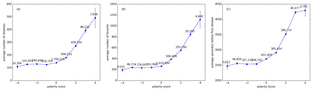
Figure 2: The effect of sentiment on information diffusion.
(A) the average number of retweets, (B) the average number of favorites, and (C) the average number of seconds passed before the first retweet, as a function of the polarity score of the given tweet. The number on the points represent the amount of tweets with such polarity score in our sample. Bars represent standard errors.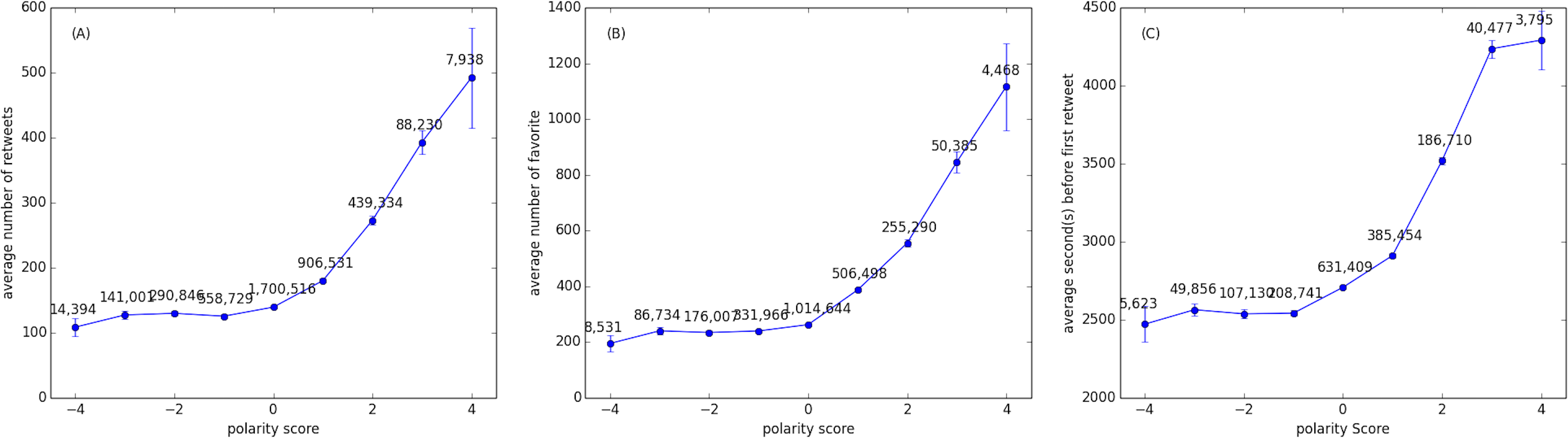
Two important considerations emerge from the analysis of Fig. 2: (i) positive tweets spread broader than neutral ones, and collect more favorites, but interestingly negative posts do not spread any more or less than neutral ones, neither get more or less favorited. This suggests the hypothesis of observing the presence of positivity bias (Garcia, Garas & Schweitzer, 2012) (or Pollyanna hypothesis (Boucher & Osgood, 1969)), that is the tendency of individuals to favor positive rather than neutral or negative items, and choose what information to favor or rebroadcast further accordingly to this bias. (ii) Negative content spread much faster than positive ones, albeit not significantly faster than neutral ones. This suggests that positive tweets require more time to be rebroadcasted, while negative or neutral posts generally achieve their first retweet twice as fast. Interestingly, previous studies on information cascades showed that all retweets after the first take increasingly less time, which means that popular content benefit from a feedback loop that speeds up the diffusion more and more as a consequence of the increasing popularity (Kwak et al., 2010).
Conversations’ dynamics and sentiment evolution
To investigate how sentiment correlates with content popularity, we now only consider active and exclusive discussions occurred on Twitter in September 2014. Each topic of discussion is here identified by its most common hashtag. Active discussions are defined as those with more than 200 tweets (in our dataset, which is roughly a 10% sample of the public tweets), and exclusive ones are defined as those whose hashtag never appeared in the previous (August 2014) and the next (October 2014) month.
Inspired by previous studies that aimed at finding how many types of different conversations occur on Twitter (Kwak et al., 2010; Lehmann et al., 2012), we characterize our discussions according to three features: the proportion pb of tweets produced within the conversation before its peak, the proportion pd of tweets produced during the peak, and finally the proportion pa of tweets produced after the peak. The peak of popularity of the conversation is simply the day which exhibits the maximum number of tweets with that given hashtag. We use the Expectation Maximization (EM) algorithm to learn an optimal Gaussian Mixture Model (GMM) in the (pb, pa) space. To determine the appropriate number of components (i.e., the number of types of conversations), we adopt three GMM models (spherical, diagonal, and full) and perform a 5-fold cross-validation using the Bayesian Information Criterion (BIC) as quality measure. We vary the number of components from 1 to 6. Figure 3B shows the BIC scores for different number of mixtures: the lower the BIC score, the better. The outcome of this process determines that the optimal number of components is four, in agreement with previous studies (Lehmann et al., 2012), as captured the best by the full GMM model. In Fig. 3A we show the optimal GMM that identifies the four classes of conversation: the two dimensions represent the proportion pb of tweets occurring before (y axis) and pa after (x axis) the peak of popularity of each conversation.
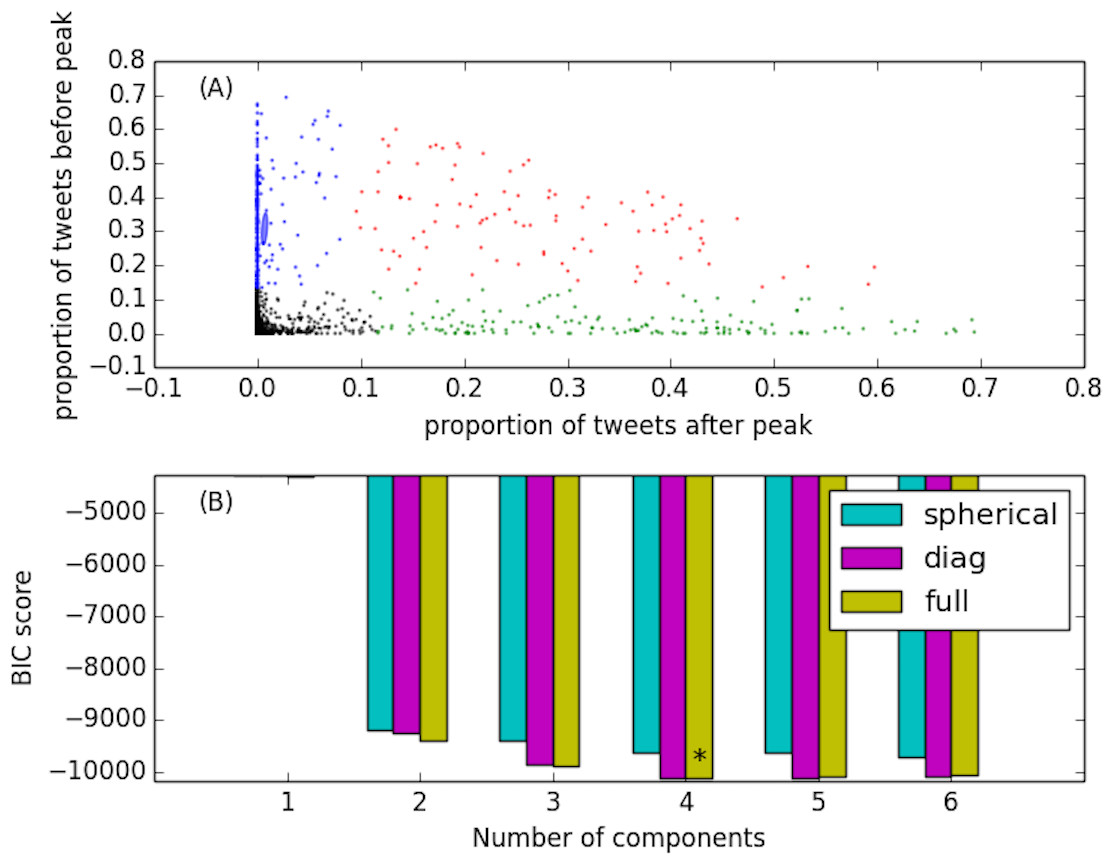
Figure 3: Dynamical classes of popularity capturing four different types of Twitter conversations.
(A) shows the Gaussian Mixture Model employed to discover the four classes. The y and x axes represent, respectively, the proportion of tweets occurring before and after the peak of popularity of a given discussion. Different colors represent different classes: anticipatory discussions (blue dots), unexpected events (green), symmetric discussions (red), transient events (black). (B) shows the BIC scores of different number of mixture components for the GMM (the lower the BIC the better the GMM captures the data). The star identifies the optimal number of mixtures, four, best captured by the full model.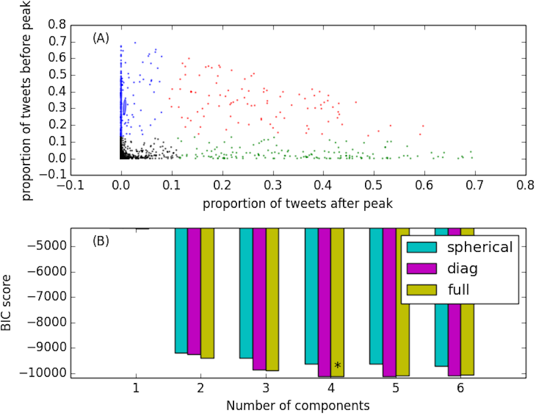
The four classes correspond to: (i) anticipatory discussions (blue dots), (ii) unexpected events (green), (iii) symmetric discussions (red), and (iv) transient events (black). Anticipatory conversations (blue) exhibit most of the activity before and during the peak. These discussions build up over time registering an anticipatory behavior of the audience, and quickly fade out after the peak. The complementary behavior is exhibited by discussions around unexpected events (green dots): the peak is reached suddenly as a reaction to some exogenous event, and the discussion quickly decays afterwards. Symmetric discussions (red dots) are characterized by a balanced number of tweets produced before, during, and after the peak time. Finally, transient discussions (black dots) are typically bursty but short events that gather a lot of attention, yet immediately phase away afterwards. According to this classification, out of 1,522 active and exclusive conversations (hashtags) observed in September 2014, we obtained 64 hashtags of class A (anticipatory), 156 of class B (unexpected), 56 of class C (symmetric), and 1,246 of class D (transient), respectively. Figure 4 shows examples representing the four dynamical classes of conversations registered in our dataset. The conversation lengths are all set to 7 days, and centered at the peak day (time window 0).
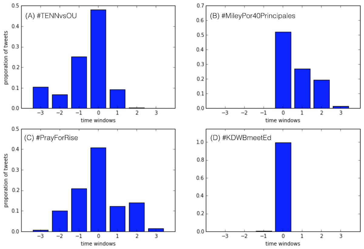
Figure 4: Example of four types of Twitter conversations reflecting the respective dynamical classes in our dataset.
(A) shows one example of anticipatory discussion (#TENNvsOU); (B) an unexpected event (#MileyPor40Principales); (C) a symmetric discussion (#PrayForRise); and (D) a transient event (#KDWBmeetEd).
Figure 4A represents an example of anticipatory discussion: the event captured (#TENNvsOU) is the football game Tennessee Volunteers vs. Oklahoma Sooners of Sept. 13, 2014. The anticipatory nature of the discussion is captured by the increasing amount of tweets generated before the peak (time window 0) and by the drastic drop afterwards. Figure 4B shows an example (#MileyPor40Principales) of discussion around an unexpected event, namely the release by Los 40 Principales of an exclusive interview to Miley Cyrus, on Sept. 10, 2014. There is no activity before the peak point, that is reached immediately the day of the news release, and after that the volume of discussion decreases rapidly. Figure 4C represents the discussion of a symmetric event: #PrayForRise was a hashtag adopted to support RiSe, the singer of the K-pop band Ladies’ Code, who was involved in a car accident that eventually caused her death. The symmetric activity of the discussion perfectly reflects the events1: the discussion starts the day of the accident, on September 3, 2014, and peaks the day of RiSe’s death (after four days from the accident, on September 7, 2014), but the fans’ conversation stays alive to commemorate her for several days afterwards. Lastly, Fig. 4D shows one example (#KDWBmeetEd) of transient event, namely the radio station KDWB announcing a lottery drawing of the tickets for Ed Sheeran’s concert, on Sept. 15, 2014. The hype is momentarily and the discussion fades away immediately after the lottery is concluded.
Figure 5 shows the evolution of sentiment for the four classes of Twitter conversations: it can be useful to remind the average proportions of neutral (42.46%), positive (35.95%), and negative (21.59%) sentiments in our dataset, to compare them against the distributions for popular discussions. Also worth noting, although each discussion is hard-cast in a class (anticipatory, unexpected, symmetric, or transient), sometimes spurious content might appear before or after the peak, causing the presence of some small amount of tweets where ideally we would not expect any (for example, some tweets appear after the peak of an anticipatory discussion). We grayed out the bars in Figs. 5A, 5B and 5D, to represent non-significant amounts of tweets that are present only as byproduct of averaging across all conversations belonging to each specific class. These intervals therefore do not convey any statistically significant information and are disregarded. (A) For anticipatory events, the amount of positive sentiment grows steadily until the peak time, while the negative sentiment is somewhat constant throughout the entire anticipatory phase. Notably, the amount of negative content is much below the dataset average, fluctuating between 9% and 12% (almost half of the dataset average), while the positive content is well above average, ranging between 40% and 44%. This suggests that, in general, anticipatory popular conversations are emotionally positive. (B) The class of unexpected events intuitively carries more negative sentiment, that stays constant throughout the entire discussion period to levels of the dataset average. (C) Symmetric popular discussions are characterized by a steadily decreasing negative emotions, that goes from about 23% (above dataset’s average) at the inception of the discussions, to around 12% toward the end of the conversations. Complementary behavior happens for positive emotions, that start around 35% (equal to the dataset average) and steadily grow up to 45% toward the end. This suggests that in symmetric conversations there is a general shift of emotions toward positiveness over time. (D) Finally, transient events, due to their short-lived lengths, represent more the average discussions, although they exhibit lower levels of negative sentiments (around 15%) and higher levels of positive ones (around 40%) with respect to the dataset’s averages.
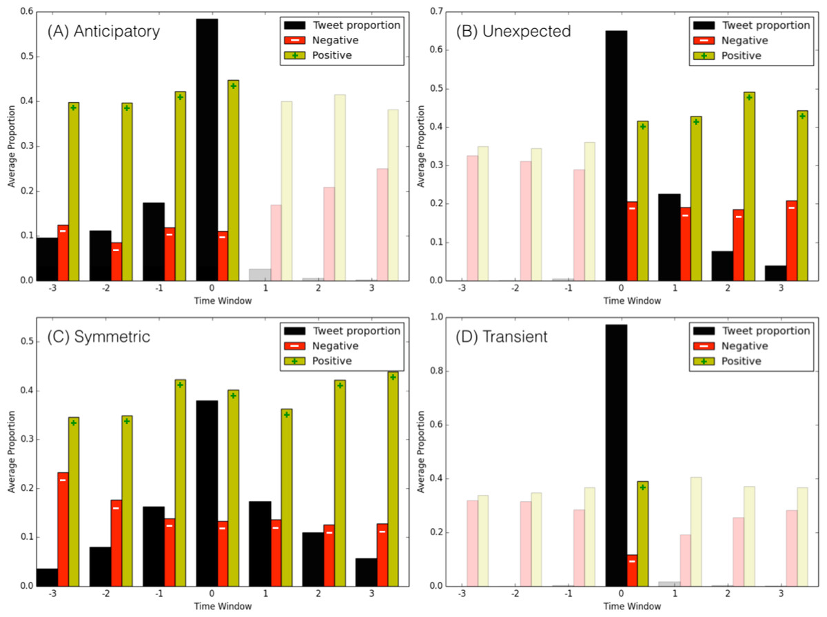
Figure 5: Evolution of positive and negative sentiment for different types of Twitter conversations.
The four panels show the average distribution of tweet proportion, and the average positive (S ≥ 1) and negative (S ≤ − 1) tweet proportions, for the four classes respectively: (A) anticipatory discussion; (B) unexpected event; (C) symmetric discussion; and, (D) transient discussion.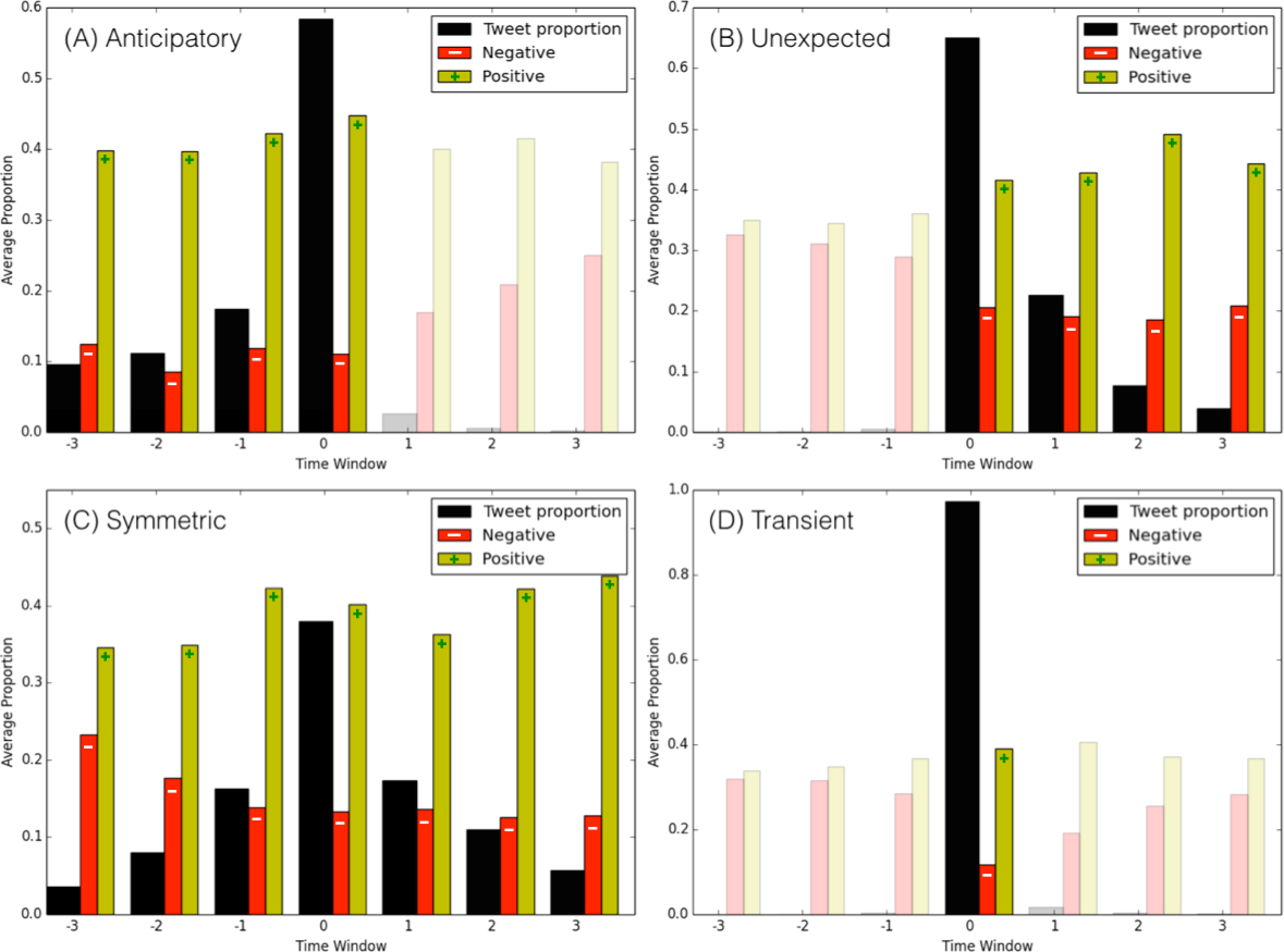
Discussion
The ability to computationally annotate at scale the emotional value of short pieces of text, like tweets, allowed us to investigate the role that emotions and sentiment expressed into social media content plays with respect to the diffusion of such information.
Our first finding in this study sheds light on how sentiment correlates with the speed and the reach of the diffusion process: tweets with negative emotional valence spread faster than neutral and positive ones. In particular, the time that passes between the publication of the original post and the first retweet is almost twice as much, on average, for positive tweets than for negative ones. This might be interpreted in a number of ways, the most likely being that content that conveys negative sentiments trigger stronger reactions in the readers, some of which might be more prone to share that piece of information with higher chance than any neutral or positive content. However, the positivity bias (or Pollyanna effect) (Garcia, Garas & Schweitzer, 2012; Boucher & Osgood, 1969) rapidly kicks in when we analyze how many times the tweets become retweeted or favorited: individuals online clearly tend to prefer positive tweets, which are favorited as much as five times more than negative or neutral ones; the same holds true for the amount of retweets collected by positive posts, which is up to 2.5 times more than negative or neutral ones. These insights provide some clear directives in terms of best practices to produce popular content: if one aims at triggering a quick reaction, negative sentiments outperform neutral or positive emotions. This is the reason why, for example, in cases of emergencies and disasters, misinformation and fear spread so fast in online environments (Ferrara et al., 2014). However, if one aims at long-lasting diffusion, then positive content ensures wide reach and the most preferences.
The second part of our study focuses on entire conversations, and investigates how different sentiment patterns emerge from discussions characterized by different temporal signatures (Kwak et al., 2010; Lehmann et al., 2012): we discover that, in general, highly-anticipated events are characterized by positive sentiment, while unexpected events are often harbingers of negative emotions; yet, transient events, whose duration is very brief, represent the norm on social media like Twitter and are not characterized by any particular emotional valence. These results might sound unsurprising, yet they have not been observed before: common sense would suggest, for example, that unprecedented conversations often relate to unexpected events, such as disasters, emergencies, etc., that canalize vast negative emotions from the audience, including fear, sorrow, grief, etc. (Sakaki, Okazaki & Matsuo, 2010). Anticipated conversations instead characterize events that will occur in the foreseeable future, such as a political election, a sport match, a movie release, an entertainment event, or a recurring festivity: such events are generally positively received, yet the attention toward them quickly phases out after their happening (Lehmann et al., 2012; Mestyán, Yasseri & Kertész, 2013; Le, Ferrara & Flammini, 2015). Elections and sport events might represent special cases, as they might open up room for debate, “flames”, polarized opinions, etc. (Ratkiewicz et al., 2011; Bond et al., 2012) (such characteristics have indeed been exploited to make predictions (Asur & Huberman, 2010; Metaxas & Mustafaraj, 2012; Le, Ferrara & Flammini, 2015)).
The findings of this paper have very practical consequences that are relevant both for economic and social impact: understanding the dynamics of information diffusion and the effect of sentiment on such phenomena becomes crucial if one, for example, wants to craft a policy to effectively communicate with an audience. The applications range from advertisement and marketing, to public policy and emergency management. Recent events, going for tragic episodes of terrorism, to the emergence of pandemics like Ebola, have highlighted once again how central social media are in the timely diffusion of information, yet how dangerous they can be when they are abused or misused to spread misinformation or fear. Our contribution pushes forward previous studies on sentiment and information diffusion (Dang-Xuan & Stieglitz, 2012) and furthers our understanding of how the emotions expressed in a short piece of text might correlated with its spreading in online social ecosystems, helping to craft effective information diffusion strategies that account for the emotional valence of the content.