
Optimal robust configuration in cloud environment based on heuristic optimization algorithm
- Published
- Accepted
- Received
- Academic Editor
- Bilal Alatas
- Subject Areas
- Distributed and Parallel Computing, Theory and Formal Methods
- Keywords
- Cloud computing, Robustness, Waiting time, Profit
- Copyright
- © 2024 Zhou et al.
- Licence
- This is an open access article distributed under the terms of the Creative Commons Attribution License, which permits using, remixing, and building upon the work non-commercially, as long as it is properly attributed. For attribution, the original author(s), title, publication source (PeerJ Computer Science) and either DOI or URL of the article must be cited.
- Cite this article
- 2024. Optimal robust configuration in cloud environment based on heuristic optimization algorithm. PeerJ Computer Science 10:e2350 https://doi.org/10.7717/peerj-cs.2350
Abstract
To analyze performance in cloud computing, some unpredictable perturbations that may lead to performance degradation are essential factors that should not be neglected. To prevent performance degradation in cloud computing systems, it is reasonable to measure the impact of the perturbations and propose a robust configuration strategy to maintain the performance of the system at an acceptable level. In this article, unlike previous research focusing on profit maximization and waiting time minimization, our study starts with the bottom line of expected performance degradation due to perturbation. The bottom line is quantified as the minimum acceptable profit and the maximum acceptable waiting time, and then the corresponding feasible region is defined. By comparing between the system’s actual working performance and the bottom line, the concept of robustness is invoked as a guiding basis for configuring server size and speed in feasible regions, so that the performance of the cloud computing system can be maintained at an acceptable level when perturbed. Subsequently, to improve the robustness of the system as much as possible, discuss the robustness measurement method. A heuristic optimization algorithm is proposed and compared with other heuristic optimization algorithms to verify the performance of the algorithm. Experimental results show that the magnitude error of the solution of our algorithm compared with the most advanced benchmark scheme is on the order of 10−6, indicating the accuracy of our solution.
Introduction
Today, cloud computing has developed into an integral part of current and future information technology. Cloud services are widely used by many organizations and individual users due to the presence of various advantages such as high efficiency (Sana & Li, 2021), reliability (Zhu et al., 2021) and low cost (Jayaprakash et al., 2021). With the dramatic increase in cloud usage, cloud service providers are unable to provide unlimited resources for customers to cope with surging or fluctuating demands (Nawrocki & Osypanka, 2021), so cloud service providers need to improve their quality of service (QoS). However, when the service level protocol is configured to pursue QoS, the existence of perturbation factors in the cloud computing environment is often unavoidable, which always brings undesired effects to the system. For this reason, cloud service providers must deal with these perturbations while maintaining high QoS and profitability. This study discusses a key industry challenge: how to configure cloud resources to ensure robustness to these perturbations. This research is consistent with the mainstream technology trends that emphasize the need for resilience and adaptive cloud infrastructure to handle dynamic and uncertain workloads (Liu & Buyya, 2020; Zhu et al., 2023).
For this reason, it is essential to configure resources wisely in the cloud environment so that customers’ demands and expectations of cloud service providers are largely met. Although the existing research has made significant progress in resource optimization in multi-server queuing models and cloud computing environments (Kumar et al., 2021), there are still the following shortcomings: Firstly, most studies assume an ideal environment and do not fully consider the actual perturbation factors (Devarasetty & Reddy, 2021; Chen, Du & Xiao, 2021). Secondly, the existing methods often lack robustness in the face of a dynamic changing environment (Belgacem, 2022; Somasundaram, 2021). For this reason, in this article, the concept of robustness is introduced into cloud computing by referring to the mathematical ideas in literature (Ali et al., 2004) when allocating resources. It aims to provide practical solutions for cloud service providers to help them achieve stable service quality and operational benefits in a dynamic environment.
According to our survey, when considering perturbations in the cloud environment, we can reasonably believe that they are reflected in four aspects: server failure, end of sleep, bandwidth sharing, and voltage fluctuation. Correspondingly, for the system, the importance of solving server failures lies in the fact that they may interrupt the service, resulting in data loss and longer response times. Therefore, it is necessary to improve the fault tolerance of the system and reduce the impact of faults on service availability (Yang & Kim, 2022). When the server is awakened from sleep, latency and performance overhead may be introduced. Therefore, optimizing the wake-up process is the key ensuring the efficient operation of the system, which can reduce the wake-up time and improve the system response speed (Gu et al., 2018). Bandwidth sharing among multiple additional tenants can lead to unpredictable network performance and congestion. It affects the QoS of applications that require consistent and high-speed data transmission. This means that a reasonable bandwidth allocation strategy is essential to maintain system performance and user satisfaction (Mohammadani et al., 2023). The sudden fluctuation of the power supply voltage may cause hardware failure, resulting in service interruption, and affecting the response time and throughput of the system. This requires effectively alleviating the negative impact of voltage fluctuations, thereby improving service stability and reliability (AL-Jumaili et al., 2021).
When referring to the former two and latter two cases, server size (i.e., the number of servers) and server speed (i.e., the speed of servers) will encounter unexpected changes respectively. According to the above considerations, once the expectation of cloud service provider towards the lower limit of profit and the one of customers towards the upper limit of waiting time are determined, those fluctuations in the number and speed of servers will lead to unsatisfactory results of cloud service providers and customers about their expectation. Therefore, the impact of perturbations should be fully considered when configuring the cloud platform.
In this article, to meet the expectations of cloud service providers and customers from the impact of the perturbations, a suitable configuration of the resources in the cloud platform can be considered as ensuring the robustness of the cloud computing system. On this basis, three questions are elicited. First, how to model the cloud environment with perturbations? Second, how to perform robustness metrics on it? Third, how to obtain the optimal configuration to ensure robustness?
When addressing the first question, some discussions about the impact of the perturbations on resource allocation problems have been investigated. For example, Gong et al. (2019) proposed an adaptive control method of resource allocation considering perturbations to adaptively respond to the dynamic requests of workload and resource requirements, and ensure QoS in the case of an insufficient resource pool. Wang et al. (2022b) proved the stability of manifold neural networks (MNNs) resource allocation strategies under absolute perturbations to the Laplace-Beltrami operator, representing the manifold of system noise and dynamics present in wireless systems. Hui et al. (2019) investigated a resource allocation mechanism based on a deterministic differential equation model and extended it to a mobile-edge computing (MEC) network environment with stochastic perturbations to develop a new stochastic differential equation model. The relationship between the oscillation and the intensity of the stochastic perturbation is quantitatively analyzed. These works provide us with the idea of considering the existence of perturbations in resource allocation.
When referring to the second question, it is well known that the robustness of the system is a very extensive topic in the control field. For example, Xu et al. (2021) studied the tracking control problem for a class of uncertain strict-feedback systems with robust design and learning systems. Experiments show that the proposed method is robust and adaptive to system uncertainties. Wang, Li & Chen (2019) solved the problem of robust adaptive finite-time tracking control for a class of mechanical systems in the presence of model uncertainty, unknown external perturbations, and input nonlinearity including saturation and dead zones. Although various studies have been conducted on the concept of robustness in control systems, only a few researches can be found in cloud computing systems. For instance, Yang et al. (2022) proposed a heuristic-based optimal selection method to enhance the robustness of composite manufacturing services in the planning phase of the cloud manufacturing process. Smara et al. (2022) proposed a new formalized framework for using the distributed recovery block (DRB) scheme to build reliable and usable cloud components. Cloud reliability is improved by building fault shielding nodes to uniformly handle software and hardware failures. Chen et al. (2020a) proposed a robust computational offloading strategy with fault recovery in small cloud systems with intermittent connectivity, aiming to reduce energy consumption and shorten application completion time. These references provide us with inspiration to discuss robustness issues in the cloud environment.
When referring to the third question, the optimal configuration of the resources in cloud computing systems attracts much attention. For example, Kaur (2021) proposed a new three-tier architecture to manage resources in an economic cloud marketplace, taking into account the deadline and execution time of customer tasks. Zhang et al. (2024) achieved dynamic provisioning of distributed resources in cloud manufacturing (CMfg) while reducing overall completion time and improving resource utilization, taking into account random order arrivals. Khan (2021) proposed a dynamic virtual machine (VM) consolidation approach based on load balancing to minimize trade-offs between energy consumption, SLA violations, and VM migration, while maintaining minimal host shutdowns and low time complexity in heterogeneous environments. Devarasetty & Reddy (2021) proposed an improved resource allocation optimization algorithm considering the objectives of minimizing deployment cost and improving QoS performance customers’ requirements of QoS are considered and resources are allocated within a given budget. Durgadevi & Srinivasan (2020) proposed a hybrid optimization algorithm where request speed and size are evaluated and used to allocate resources on the server side in a given system. These works provide a reference for us to solve the optimal configuration problem.
Considering the recognized deficiencies in the allocation of processing resources during perturbations, the research questions of this study are crucial. This research provides practical insights and strategies for cloud service providers to achieve a balance between QoS and profit under dynamic conditions, especially in the face of unpredictable perturbations.
The main contributions of this article are summarized as follows:
-
Defined the bounded constraints on profit and average waiting time to reflect the worst-case scenario acceptable to cloud service providers and customers, taking into account perturbations.
-
Defined the concept of robust radius to force the shortest distance between the actual configuration and the boundary to be maximized.
-
Proposed an optimal robust configuration scheme to obtain the optimal configuration of server size and speed in the presence of unpredictable perturbations.
-
Performed a series of algorithms and experimental comparisons to validate the scheme.
The remainder of this article is organized as follows. ‘Related work’ provides a review of related work. ‘Materials and methods’ constructs the cloud computing system as a multi-server queuing model, derives the models of profit and average waiting time, clarifies the optimization problem and robustness metric. ‘Optimal robust configuration’ presents the optimal robust configuration scheme and validates the performance of the algorithm. ‘Results’ further verifies the result of the scheme. ‘Discussion’ analyzes the significance and defects of this work. ‘Conclusion’ concludes this work.
Related Work
In this section, we first review the recent works relevant to the modeling problem of the queuing system. Subsequently, we review the recent work related to the problem of profit maximization and then review the work related to optimizing the waiting time in cloud systems.
While considering the queuing systems with multiple stages, Kim, Kim & Bueker (2021) studied the customer equilibrium strategy and the optimal priority cost associated with social cost minimization for an unobservable M/M/m queue with two priority categories and multiple vacations. Adhikari et al. (2021) used the M/M/c queuing model to compare the average waiting time, and analyzed the server utilization to reduce the overall waiting time and server utilization. Mrhaouarh, Namir & Chafiq (2021) considered a stable M/M/m multi-server parallel working model to optimize the cost to achieve maximum profit in the cloud computing environment. Kapgate (2023) proposed a data center (DC) selection algorithm based on request–response time prediction. The results of the DC selection optimization function based on M/M/m queuing theory are used to minimize the response time of the whole system.
When discussing the profit maximization problem in cloud computing, some researches are investigated under specific constraints. For example, Swain, Gupta & Sahu (2020) proposed the constraint-aware profit-ranking and mapping heuristic algorithm for efficient scheduling of tasks to obtain maximum profit. Cong et al. (2022) proposed an efficient grouped gray wolf optimizer-based heuristic method, which determined the optimal multi-server configuration for a given customer who demands to maximize the profitability of cloud services. Wang et al. (2023) presented a resource collaboration and expanding scheme, which maximized long-term profitability and maintained computational latency. Najm & Tamarapalli (2020) proposed an algorithm for migrating virtual machines between data centers in a federated cloud, through which the operational costs of cloud providers were reduced. Du, Wu & Huang (2019) used a black-box approach and leveraged model-free deep reinforcement learning, through which the dynamics of cloud subscribers were captured and the cloud provider’s net profit was maximized. All of these researches can effectively help us choose the appropriate method to discuss the profit maximization problem.
Apart from the profit maximization problem, the waiting time of customers, as an important issue reflecting the efficiency of the service and the customers’ attitude, simultaneously affecting the level of customers’ satisfaction with the quantity of service, is also worthy of discussing. For example, Belgacem, Mahmoudi & Kihl (2022) proposed a new intelligent multi-agent system and reinforcement learning method (IMARM), which made the system with reasonable load balance as well as execution time by moving the virtual machines to the optimal state. Soulegan, Barekatain & Neysiani (2021) proposed an optimization method based on a multipurpose weighted genetic algorithm to minimize the parameters such as waiting time and cost. Rajakumari et al. (2022) proposed a fuzzy hybrid particle swarm parallel ant colony optimization approach on cloud computing to achieve improved task scheduling by minimizing execution and waiting time, system throughput, and maximizing resource utilization. Shadi et al. (2021) provided a cloud-assisted ready-time partitioning technique that precisely partitions each task in a customer’s work-flow as it becomes ready. The technique aims to minimize the energy consumption of each mobile user device while meeting user-defined deadlines. Vijaya Krishna, Ramasubbareddy & Govinda (2020) used and implemented a mixture of shortest job priority and scheduling based priority in cloud environment. The average waiting time and turnaround time were greatly reduced. Besides, the efficiency of cloud resource management was significantly improved. According to the supply–demand relationship between cloud service providers and customers, profit maximization and waiting time are the primary concerns of both parties, respectively. For this reason, in our robustness discussion for cloud environment where perturbation is presented, these two aspects are considered simultaneously.
Materials and Methods
The models
Multi-server system
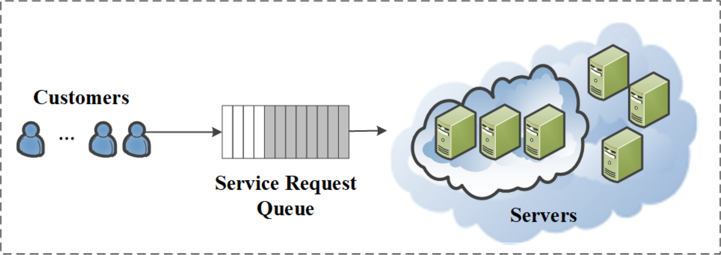
Portions of this text were previously published as part of a preprint (Zhou, Chen & Kuang, 2023). In this article, we consider an M/M/m multi-server queuing system, which is shown in Fig. 1. The notations used are listed in Table 1. For the multi-server system, it has m identical servers with speed s (hundred billion instructions per hour). When a customer arrives the queue with service requests, it will be served immediately as long as any server is available. Due to the randomness of the arrival of the customers, we consider the time it takes customers to arrive at the system as a random variable with an independent and identically distributed (i.i.d.) exponential distribution whose mean is 1/λ. In other words, the service requests follow a Poisson process with arrival rate λ. The task execution demand is measured by the number of instructions, which can be denoted by a the exponential random variable j with mean . Thus, the execution time of a task on the multi-server system can also be considered as an exponential random variable t = j/s with mean . Moreover, the service rate can be denoted as and the utilization factor is defined as , which means the percentage of the average time when the server is in busy state. Since the total number of service requests brought by customers is M, which determines the upper limit of the service requests being waited or processed in the M/M/1//M queuing system, Let pk denotes the probability that there are k service requests (waiting or being processed) in the M/M/m queuing system. Then, we have
(1)where (2)
To ensure the ergodicity of queue system, it is obviously that the condition 0 < ρ < 1 should be satisfied.

Figure 1: Multi-server queuing system (Chen et al., 2020b).
| Symbol | Definition | Symbol | Definition |
|---|---|---|---|
| λ | The number of arrival customer per (unit time) UT | j | Task execution demand |
| m | Server size | s | Server speed |
| µ | The number of completed service per UT | ρ | The utilization factor of servers |
| Pk | The probability that k service requests in system | Pq | The probability to wait |
| W | Waiting time of customers | fw(t) | The pdf of waiting time |
| u(t) | Unit impulse function | T | The expectation of waiting time |
| ɛ | Revenue | C | Cost |
| G | Profit of cloud service providers | a | Fees per one billion instructions |
| D | Maximum tolerable time that customers can wait | β | Rental price of a server per UT |
| Nsw | Average gate switching factor per clock cycle | Cl | Load capacitance |
| V | Supply voltage | f | Lock frequency |
| ϕ | A positive constant | b | A positive proportional coefficient |
| Pd | Dynamic power consumption | P∗ | Static power consumption |
| δ | Electricity price of energy | H∗ | A working point in feasibel region |
| H | A point on boundary | r | Shortest robustness radius |
| θ | Polar angle in vector form | r1 | Step length of neighborhood search |
| 11 | Indicator function 1 | sz | optimal server size |
| 12 | Indicator function 2 | mz | optimal server speed |
On this basis, when all servers in a multi-server system are occupied by executing service requests, newly arrived service requests must wait in the queue. We express the probability (i.e., the probability that a newly arrived service request have to wait) as follows. (3)
Waiting time distribution
When enjoying the services, customers always want to have shorter waiting time. Therefore, it is necessary to model the waiting time of customers, such that it can be better quantified. With this premise in mind, we denote W as the waiting time of the service request arriving at the multi-server system. Notice that, the probability distribution function (pdf) of waiting time in M/M/m queuing system has already been fully considered in previous literatures, which is shown as follow Mei et al. (2018). (4) where and is unit impulse function, which is defined as (5)
The function has the following property (6)
namely, can be treated as a pdf of a random variable with expectation (7)
Let z → ∞ and define . It is clear that any random variable whose pdf is has expectation 0.
Further, according to Eqs. (4) and (6), we can calculate the expectation of waiting time as follow. (8)
Profit modeling
Cloud service providers play an important role in maintaining the cloud service platform as well as serving customer requests. During the operation of the platform, for the cloud service provider, revenue can be obtained from the customers whose requests have to be served, while operational costs have to be paid for maintaining the platform. In this article, we denote ɛ and C as the revenue and the cost of cloud service provider respectively. Subtracting the former to the latter, the profit of cloud service provider can be obtained, which can be demonstrated in Eq. (9). (9) where, G is the profit obtained by cloud service provider. In the following subsections, the revenue and cost of cloud service provider will be modeled in detail.
Revenue modeling.
The customers have to pay for the services provided by the cloud service provider. To evaluate the relationship between the quality of services and the corresponding charges to the customers, SLA is adopted. In this article, we use flat rate pricing for service requests because it is relatively intuitive and easy to be obtained. Based on this, the service charge function R can be expressed as (10)
where a is a constant that represents the fee per unit service, D is the maximum tolerable time that a service request can wait (i.e., the deadline). In this article, when the waiting time does not exceed the maximum value, the fee that the customer will pay is considered as a constant value. Otherwise, the customer will enjoy the services for free.
Based on Eqs. (4) and (10), we can calculate the expectations of R(j, W) (11)
Notice that, the task execution requirement j is also a random variable, which follows the exponential distribution. On this basis, the expected charge of a service request in multi-server system can be calculated as follow. (12)
Further, we can also obtain (13)
Since the number of service requests arriving the multi-server system is λ per UT, the total revenue of cloud service provider is if all the service requests could be served before the deadline. However, if parts of the service requests are served for free, the actual revenue earned by the cloud service provider can be described as (14)
Cost modeling.
The costs to the cloud service provider consists of two main components, namely the cost of infrastructure leasing and energy consumption. The infrastructure provider maintains a large number of servers for loan, and the cloud service provider rents the servers on request and pays the corresponding leasing fees. Assume that the rental price of one server per UT is β, then the server rental price of m multi-server system is mβ.
The cost of energy consumption, another part of the service provider’s cost, consists of the price of electricity and the amount of energy consumed. In this article, the following dynamic power model is used to express the energy consumption, which has been discussed in much of the literature Li et al. (2021). (15) where Nsw is the average gate switching factor per clock cycle, CL is the load capacitance, V is the supply voltage, and f is the clock frequency.
In the ideal case, the relationship between the supply voltage V and the clock frequency f can be described as V ∝ fϕ . The execution server speed s is usually linearly related to the clock frequency, namely, s ∝ f. Therefore, the dynamic power model can be converted to Pd ∝ bNswCLs2ϕ+1. For the sake of simplicity, we can assume Pd = bNswCLs2ϕ+1 = ξsα, where ξ = bNswCL and α = 2ϕ + 1. In this article, we set NswCL = 4, b = 0.5, ϕ = 0.55. Hence, α = 2.1 and ξ = 2.
Apart from dynamic power consumption, it is reasonable to think that some amount of static power are consumed by the servers when they are idle. In this case, the average amount of energy consumption per unit of time can be described as P = ρξsα + P∗, where P∗ is the static power consumption.
Notice that, the necessary and sufficient condition for ergodicity in the M/M/m queuing system is ρ < 1. However, P = ρξsα + P∗ implies that ρ = 1. Therefore, the average amount of energy consumption per unit of time can be further described as P = ρξsα + P∗. Assuming an electricity price of δ per watt, the total cost per UT for the cloud service provider can be described as (16)
Problem description
In order to solve the problem of robust configuration in cloud environment, we propose a performance-aware robust configuration strategy, as shown in Algorithm 1 (Wang, Li & Ruiz, 2019). The algorithm consists of three parts: (i) determining the tolerable feasible region of the discussion. (ii) obtaining the robust radius r from the working point to the boundary. (iii) discussing the three possible robustness problems in detail.
_______________________
 Algorithm 1: Performance-aware robust configuration strategy        _________
  1  begin
     2   Set the feasible region according to the robustness analysis.
3   Obtain the robustness radius r from working point to the boundary;
4   if deadline aware configuration then
    5   Obtain T-feasible region using Equation (19)
6   Calculate r using Equation (23)
7   Call r according to the Robust configuration method;
8   else if profit aware configuration then
    9   Obtain D-feasible region using Equation (21);
10   Calculate r using Equation (23);
11   Call r according to the Robust configuration method;
12   else
    13   Obtain T-feasible region and G-feasible region using
Equations (19)(21);
14   Calculate r using Equation (23);
15   Call r according to the Robust configuration method;
16   end
17  end
Robustness analysis
Considering the demands of cloud service providers and customers described in the previous section, most researches have focused on achieving optimal results under certain conditions. However, to the best of our knowledge, perturbation factors have never been discussed in the modeling and solving process of this problem, which may result in some undesirable impacts for cloud service providers and customers. In this section, we will describe the impacts of specific perturbation factors on the profit of cloud service providers and the waiting time of customers, and then design a robust strategy to protect the demands of cloud service providers and customers as much as possible.
The derivation of equations Eqs. (8) and (9) gives us an initial insight into the demands of cloud service providers and customers. Based on this, we need to further quantify and analyze the perturbation factors (i.e., server size and speed, which are often discussed in references about profit and waiting time (Li et al., 2021; Wu et al., 2020; Li et al., 2020) in the system). According to Eqs. (8) and (9), because of the sophisticated structure of pm, the waiting time of customers and the profit of cloud service providers are difficult to analyzed numerically. For the sake of simplicity, the following approximations are adopted, i.e., (closed-form approximation) and (Stirling’s approximation of m!) (Wang et al., 2022a). Therefore, we get the following closed-form approximation of pm. (17)
Then, substituting Eqs. (17) into (13), we have (18)
Further, according to Eqs. (17) and (18), we can obtain the approximations of the waiting time of customers and the profit of cloud service providers as follow. (19)
and, (20)
In this article, we consider the perturbation factors as the unpredictable changes in server size and speed. Notice that, the utilization factor ρ in Eq. (20) can be expressed by . By substituting such expression of ρ into Eq. (20), and setting to 1 without loss of generality, (21)
For the sake of simplicity, Eqs. (19) and (21) can be rewritten as and respectively. Obviously, it can be found the strong nonlinear characteristics in Eqs. (19) and (21), which are adverse to the numerical analysis of such formulas. In this case, we choose to draw the graphics of and to show the functional relationship intuitively.
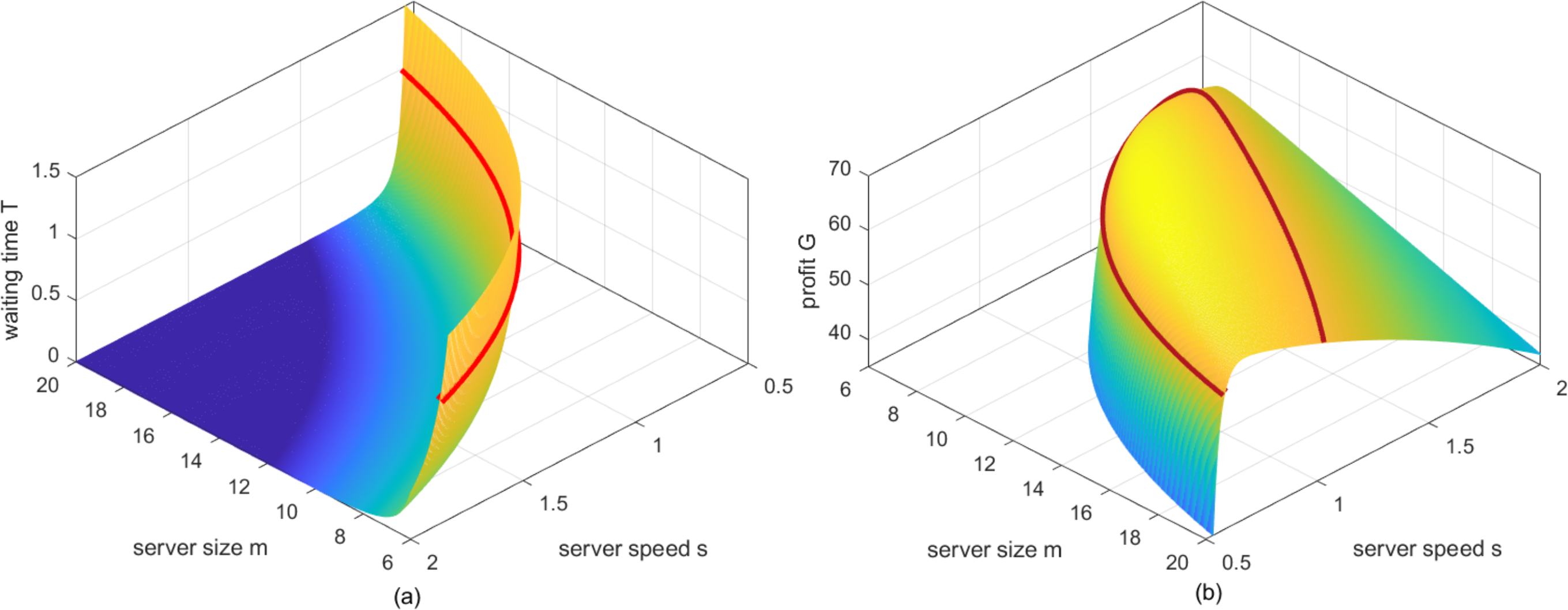
By setting λ = 10 hundred service requests per hour, a = 10 dollars per one hundred billion instructions (Note: The monetary unit “dollars” in this article may not be identical but should be linearly proportional to the real US dollars.), β = 1.5 dollars per one hundred billion instructions, δ = 0.1 and P∗ = 2, and then traversing m ∈ [6, 20], s ∈ [0.5, 2], two surfaces with respect to Eqs. (19) and (21), are shown in Figs. 2A and 2B respectively. As can be seen from Fig. 2A, when server size and speed decrease simultaneously, customers have to take a longer waiting time for their requests to be served, and vice versa. While for Fig. 2B, when server size and speed are large, the service ability of the system far exceeds the demands of customers towards the services, which will lead to unnecessary waste to cloud service providers. As server size and speed decrease, the reduction in the cost will certainly increase the profit of cloud service providers. However, when server size and speed further decrease, the profit of cloud service providers will decrease instead, for the reason that the service ability is too weak to serve enough requests before the deadline, such that parts of the customers will enjoy the services for free.
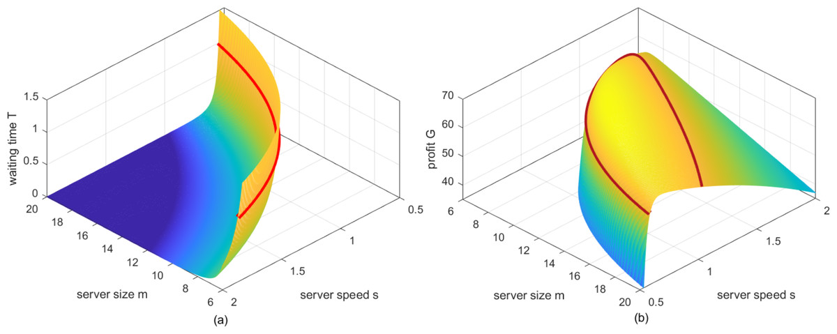
Figure 2: (A) The mesh of waiting time Tversuss and m. (B) The mesh of profit Gversuss and m.
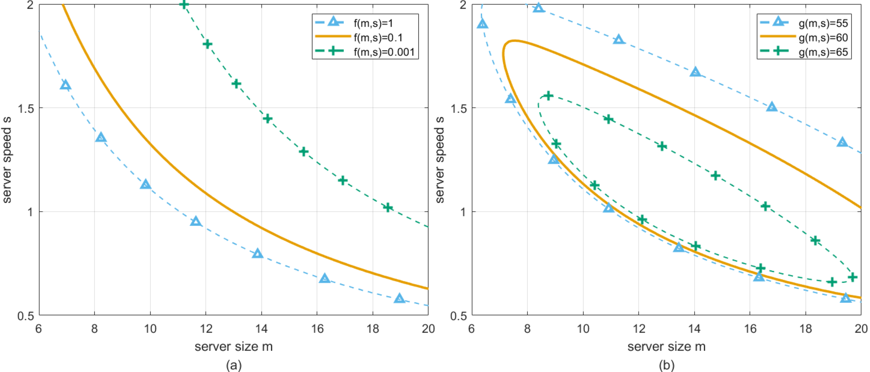
Now, refer to all the points on the surface in Fig. 2A which satisfy f(m, s) = c1, where c1 is a constant, they can be connected and shown as the red curve in Fig. 2A. Similarly, by specifying c1 ∈ [0.001, 0.1, 1], and mapping the corresponding red curves into (m, s) plane, three solid curves can be drawn in Fig. 3A. Specifically, we set the longest waiting time that customers can tolerate to be 1, which corresponds to the blue curve shown in Fig. 3A. At this time, the curve represents the bottom line of the expected performance degradation caused by the perturbation, and the region above the curve should be less than the acceptable maximum waiting time. It is obvious to find that actual server size and speed should be configured at the region above such a curve. For convenience, we refer to such region as the T-feasible region to claim the determination of such region is constrained by the waiting time of customers.
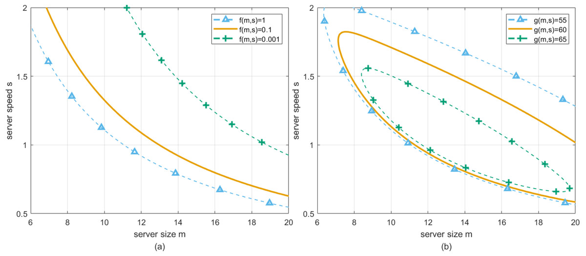
Figure 3: (A) Deadline Dversuss and m. (B) Profit Gversuss and m.
Similarly, refer to all the points on the surface in Fig. 2B that satisfy g(m, s) = c2, where c2 is a constant, they can be connected and shown as the red curve in Fig. 2B. By specifying c2 ∈ [55, 60, 65], and mapping the corresponding red curves into (m, s) plane, three solid curves can be drawn in Fig. 3B. Specifically, we set the lowest profit that cloud service providers can accept to be 55, which corresponds to the blue curve shown in Fig. 3B. At this time, the curve represents the bottom line of the expected performance degradation caused by the perturbation, and the region included in the curve should be greater than the acceptable minimum profit. It is obvious to find that actual server size and speed should be configured at the region inside this curve. For convenience, we refer to such region as the G-feasible region to claim the determination of such region is constrained by the profit of cloud service providers.
Based on the above discussion, the impacts of the perturbation factors on the profit and waiting time can be described. Now, by arbitrarily determining a point in T-feasible region, which is shown as the red point in Fig. 4A, we call such point as the working point. Namely, considering the case that perturbation is not happening, the actual configuration of server size and speed is equal to the horizontal and vertical coordinates of the red point respectively. However, once the perturbation happens, the fluctuations in server size and speed will result in the deviation of the working point. If the fluctuation is small, the configuration of server size and speed can still be located in T-feasible region. Conversely, the waiting time of customers may exceed the deadline, which is unacceptable for customers.
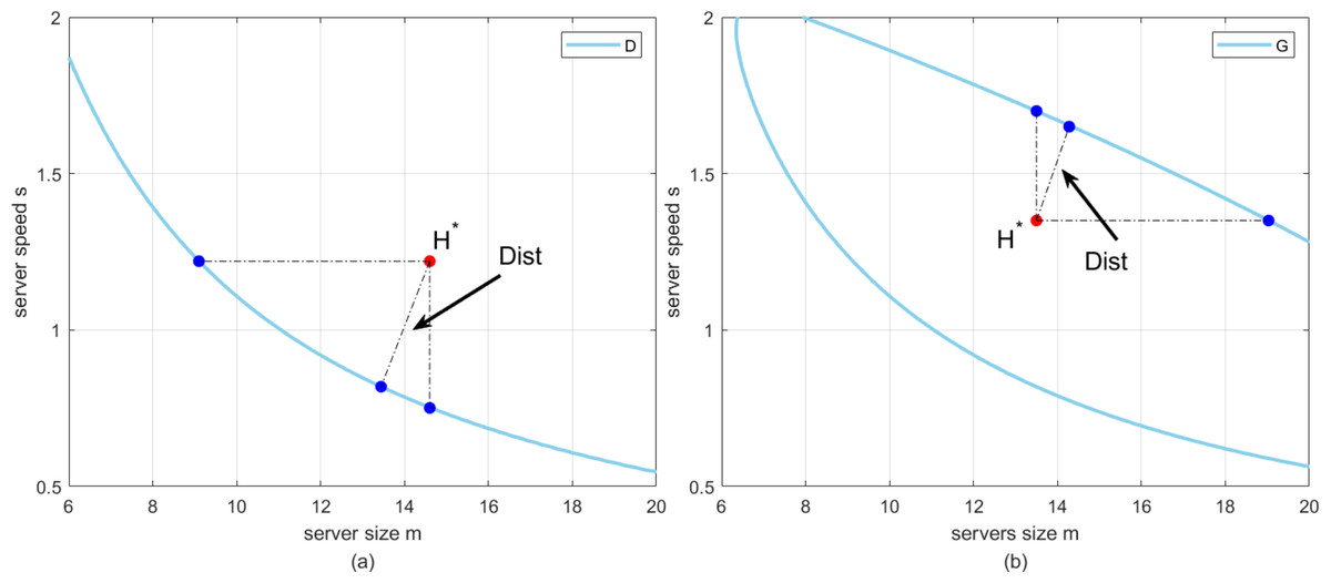
Figure 4: (A) The working pointH∗versusD. (B) The working pointH∗versusG.
Moreover, by arbitrarily determining a point in G-feasible region, which is shown as the red point in Fig. 4B, we also call such point as the working point. When the perturbation happens, the fluctuations in server size and speed will result in the deviation of the working point. If the fluctuation is small, the configuration of server size and speed can still be located in G-feasible region. Oppositely, the profit earned by cloud service providers may be less than the lowest value that they accept.
In order to overcome the shortcomings brought by those perturbations, we focus on optimizing the cloud computing system working in the worst situation, which can be explained as the idea of robustness. Benefit from such method, those cloud computing systems working in better situation will attain better performance.
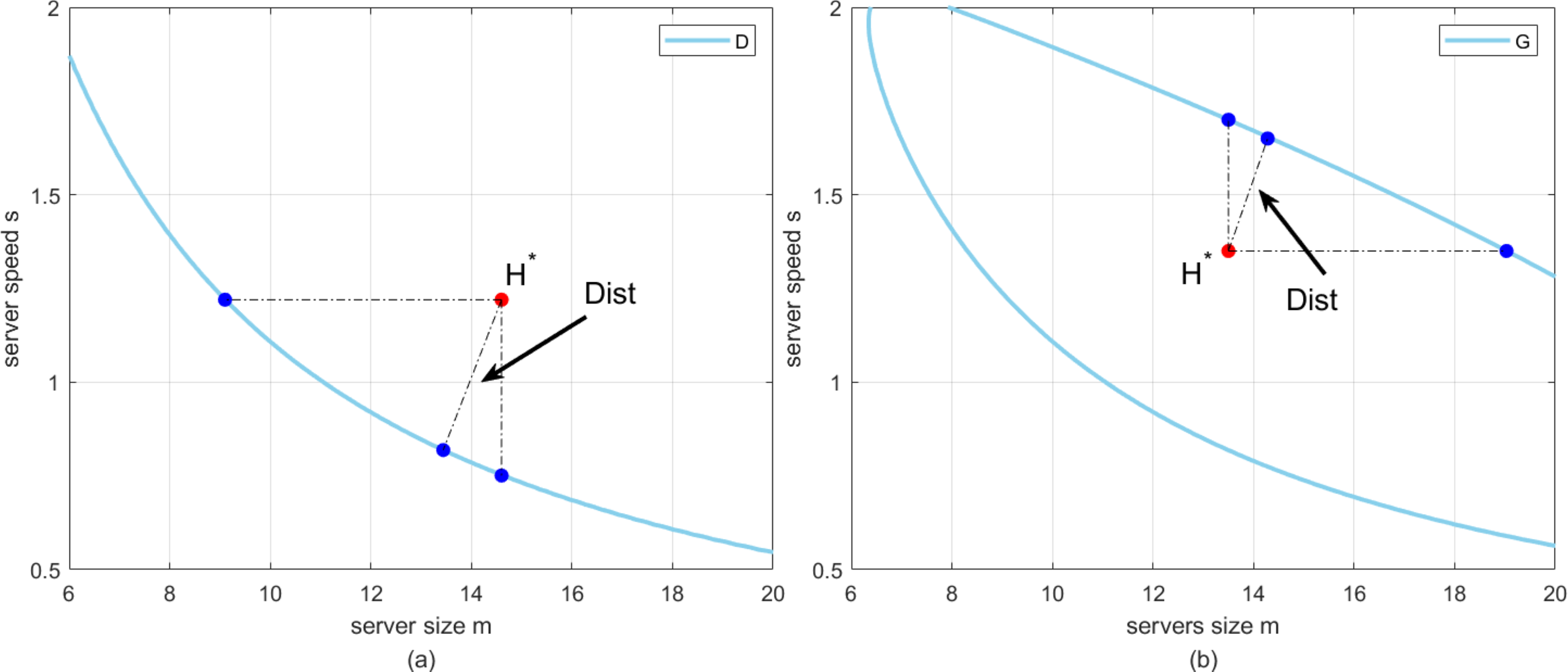
Then, we present an intuitive explanation for the idea of robustness introduced in this article. As can be seen from Figs. 4A and 4B, by denoting the working point as H∗ , and any point on the curve as H. We define the distance between H∗ and H as follow to represent the shortest distance from the working point to the boundary. (22)
Notice that, the explanations for the idea of robustness in Figs. 4A and 4B are similar. Without loss of generality, we choose the case shown in Fig. 4A as an example. For the working point arbitrarily selected in T-feasible region, we are always able to find the shortest distance between such point and the curve, which represents the worst situation that cloud computing system works in. In this article, we aim to find the optimal working point, such that the shortest distance between such point and the curve can be maximized.
Robustness metric
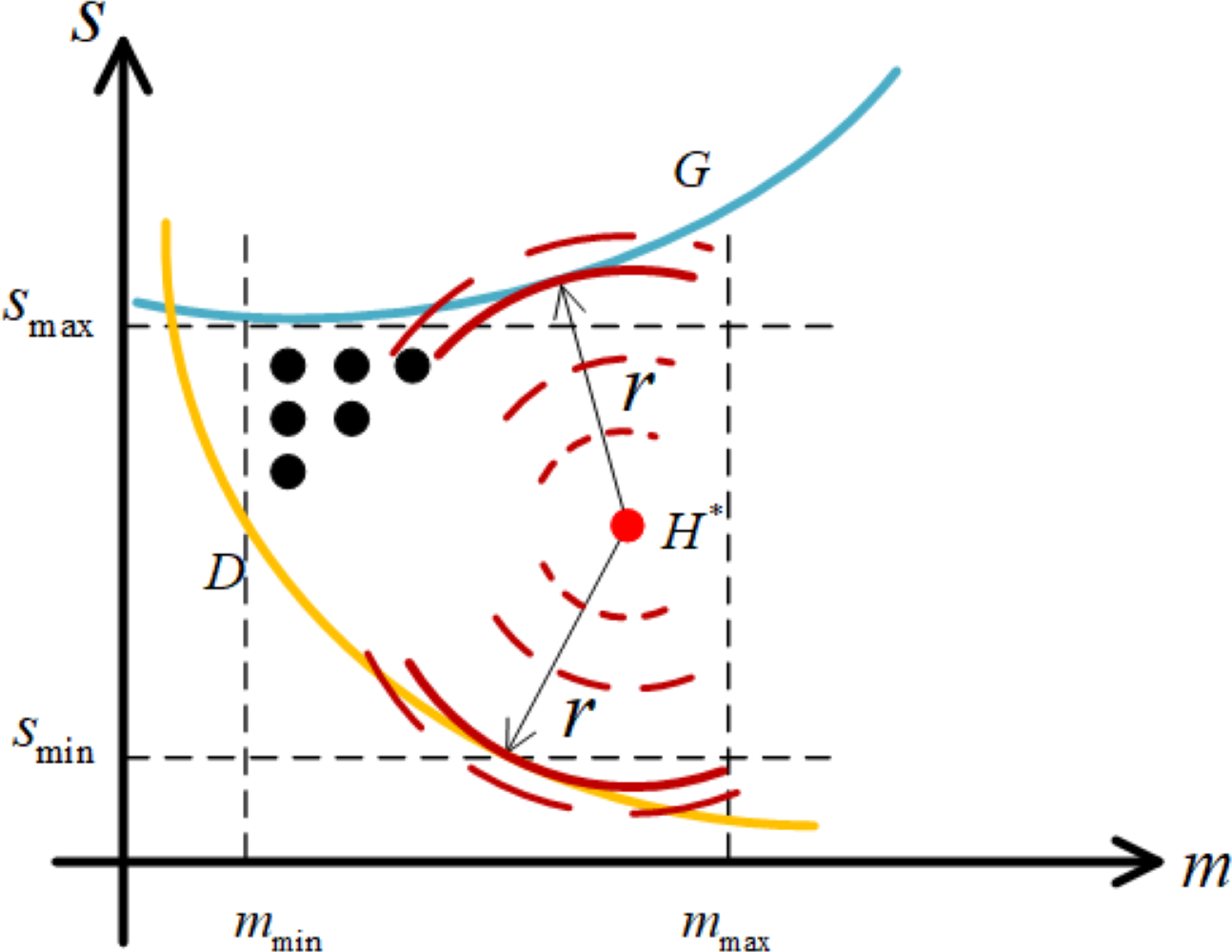
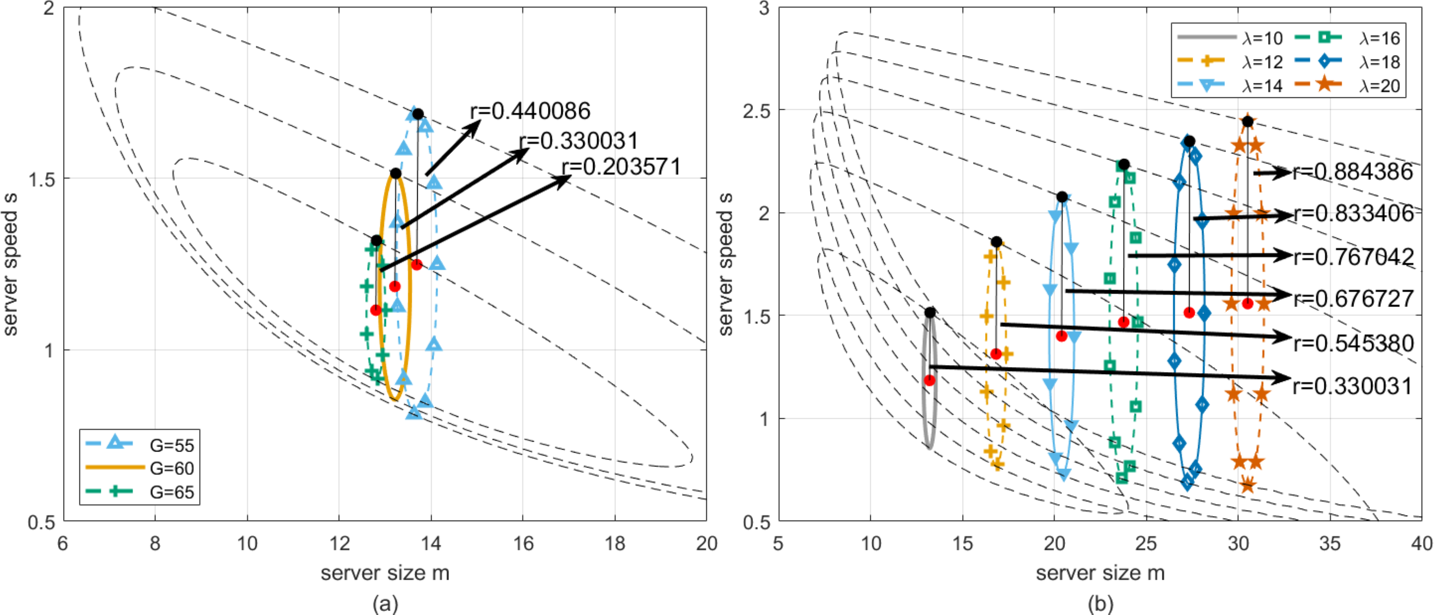
As the foundation of robustness analysis method to obtain the optimal working point, we now present a specific description for the metric of robustness in this article. For the sake of simplicity, we call the shortest distance between working point and the boundary as robustness radius, which can be formulated as follow. (23)
where H∗ and H represent the working point and the point on the boundary, respectively. Notice that, even if H∗ is determined, the analytical expression of r∗ can hardly be deduced because of the strong non-linear relationship between server size and speed by setting waiting time of customers in Eq. (19) and profit of cloud service providers in Eq. (21) to constants. Therefore, we present an intuitive graphical scheme to obtain robustness radius, which is shown in Fig. 5. Specifically, on the basis of determining the position of H∗ as the center of a circle, such circle with its radius equal to r∗ is considered as the one tangent to the boundary. In this case, the procedure for obtaining robustness radius is shown in Algorithm 2 .
__________________________________________________________________________________________
  Algorithm  2:  Neighborhood  Search  for  robustness  radius  r  from
  working point to the boundary                                                   _________
    Input:  mz, sz, l(x,y), c, 11, 12, η, ɛ, α1, α2, γ
    Output: Robustness radius rbest from working point to the boundary
  1  begin
     2   Initialization: η ← 0.1 neighborhood size; ɛ ← 10−5; β ← 0.01; α1,
    α2 ← 0.5; γ ← 0.95; r ← 0.1; rbest ← 104;
3   while |r − rbest| > ɛ do
    4   rbest ← r;
5   for θi ← 0 to 2π do
6   xi ← mz + r ⋅ cosθi;
7   yi ← sz + r ⋅ sinθi;
8   h′(xi,yi) ←−l′xi/l′yi;
9   g′(xi,yi) ←−(xi − mz)/(yi − sz);
10   end
11   F (x,y) ← h′ (x,y) − g′ (x,y);
12   F∗ (x,y) ← l (x,y) − c;
13   if arg min
     x,y    |F (x,y)| = arg min
    x,y    |F∗ (x,y)| then
   // the circle is approximately tangent to the
     boundaries
14   (xk,yk) ← arg min
    x,y    |F∗ (x,y)|;
15   if F∗ (xk,yk) > 0 then
16   r ← r + 11 ⋅ η ⋅ β − 12 ⋅ η ⋅ β;
17   else
18   r ← r − 11 ⋅ η ⋅ β + 12 ⋅ η ⋅ β;
19   end
20   else if ∑
  |F∗ (x,y)|⁄= |∑
   F∗ (x,y)| then
   // the circle intersects with the boundaries
21   r ← r − α1 ⋅ η;
22   else
   // the circle has not reached the boundaries
23   r ← r + α2 ⋅ η;
24   end
25   Updating: η ← η ⋅ γ;
26   end
27   return rbest
28 end 
Figure 5: Robustness radius r from H∗ to the boundary.
In essence, our thought strictly follows the mathematical theorems related to tangent. A tangent is a straight line that intersects the circle at exactly one point. The radius connecting the circle’s center to the tangent point is perpendicular to the tangent, which is the robustness radius we seek. Supported by this mathematical principle, the scheme for obtaining a robustness radius is further inspired by the idea of neighborhood search. Firstly, for a working point determined by its coordinates , we initialize its neighborhood, where η determines the neighborhood size, r determines the location of the neighborhood. Moreover, we also define the initial robustness radius rbest and some parameters to be used (Line 2). Then, the circulation is performed before the neighborhood converges to a certain size which is determined by the error factor ɛ (Line 3). Within each iteration, the neighborhood is discretized, and the specific operation is to collect points with the working point as the center and r as the radius of the circle (Line 5-7). Subsequently, it is necessary to calculate the slopes of two straight lines passing through those sampling points, including the slopes of the normal of their tangents (Line 8) and the slope of the straight lines both passing through these points and the center of the circle (Line 9). Please note that as complicated as the analytical expression of boundary is, the slope has to be calculated by taking the derivative of the implicit function. Specifically, by setting waiting time of customers in Eq. (19) or profit of cloud service providers in Eq. (21) to constants c, a unified form of Eqs. (19) and (21) can be deduced as l(x, y) = c with x and y represent server size and speed respectively, which clearly shows the implicit function relationship between server size and speed. Based on this, we can numerically analyze the slope matching degree (Line 11) and boundary matching degree (Line 12) of those sampling points, and then make the following judgment, where and represent slope deviation and boundary condition deviation, respectively. Worth noting, that the sampling point with zero slope deviation and zero boundary deviation obtained is a small probability event, while it can be realized to make them close to zero. In the first case, the sampling points of slope matching and boundary condition matching are the same, then it is considered that the tangent theorem is approximately satisfied, that is, the circle where the neighborhood is located has only one intersection with the boundary (Line 13-14). In this case, the point is approximately the tangent point (Line 14), and then the robustness radius is slightly adjusted according to the boundary deviation (Line 15-18). In the second case, the boundary condition deviation of the sampling point has inconsistent symbols, it is considered that the circle has exceeded the established boundary (Line 20). In this case, the radius of the next sampling should be reduced according to the size of the current neighborhood (Line 21). In the third case, the circle and the boundary have no intersection. In this case, the radius of the next sampling is increased according to the size of the current neighborhood (Line 23). Finally, as the circle tends to tangent to the boundary, the neighborhood size will gradually decrease to search more finely and ensure the convergence of the proposed scheme (Line 25).
(24) (25)Optimal robust configuration
Experiment setup
The experiment is mainly performed on a server equipped with AMD Ryzen 9 7945HX processor, 32GB memory and Windows 11. The algorithm and simulation test are implemented in MATLAB 2021b. According to our survey, the value of λ is selected in . Corresponding to different λ, the upper bounds of configurable m and s need to be adjusted, which are selected in and , respectively. Through a prior experiment, the deadline D will be selected in while the lowest acceptable profit G will be selected in .
Experiment data
The dataset utilized in this study comprises various metrics collected from a simulated cloud computing environment. The primary data points include server size and speed perturbations, instances of server failures, and bandwidth sharing metrics. The data was generated under controlled conditions to ensure robustness and statistical reliability. Each parameter was varied systematically to cover a range of real-world scenarios. This dataset forms the basis for evaluating the performance and robustness of our proposed heuristic optimization algorithm.
Experiment algorithms
In order to verify the superiority of our configuration method, we use the comparison of several heuristic algorithms provided by Zhang et al. (2022) to simulate. The results are verified by cross-validation with other algorithms and different scenarios to ensure its feasibility. Therefore, we will use the following algorithms to compare and address the problem of robust configuration in the cloud environment. The algorithms are introduced as follows:
-
Dung Beetle Optimizer (DBO) algorithm: DBO model dung beetles continuously adjust the direction and speed during the process of rolling the dung ball to ensure that the distance of the dung ball is maximized and the direction is accurate (Xue & Shen, 2022). DBO performs well in dealing with uncertainty and dynamic conditions, and can provide high-quality and robust solutions (Wang et al., 2024).
-
Egret Swarm Optimization algorithm (ESOA): ESOA updates the position by searching and capturing prey, and makes the algorithm have good diversity and balance through the cooperation and competition between individuals (Chen et al., 2022). ESOA has strong adaptability. Through cooperation and competition mechanisms, it can effectively allocate workload, improve resource utilization, and reduce response time (Yu et al., 2022).
-
Whale Optimization algorithm (WOA): WOA simulates whales to perform a random walk for global search when no prey is found, and a spiral search is performed after the prey is found (Mirjalili & Lewis, 2016). The global search ability and fast convergence characteristics of WOA enable it to effectively optimize resource allocation, reduce energy consumption and ensure service quality (Kang et al., 2022).
Experiment scenarios
Now, we call the curve that restrict T-feasible region in Fig. 3A or G-feasible region in Fig. 3B as a boundary. For any specific working point, we focus on designing an adequate algorithm to determine the shortest distance between it and the boundary. Then, some heuristic algorithms are adopted to find the optimal working point, which is equivalent to demonstrate that the horizontal and vertical coordinates of such point can be chosen to configure server size and speed in cloud computing system with greatest robustness.
For cloud computing systems, perturbation is ubiquitous. Therefore, considering the factors of perturbation, the requirements of cloud service providers and customers should be emphasized to ensure the long-term operation of cloud computing systems. In Fig. 6, the robustness analysis of the optimal working point in both T-feasible region and G-feasible region is considered. Specifically, four subgraphs can be found in this graph, which represent the four cases of interaction between T-feasible region and G-feasible region.
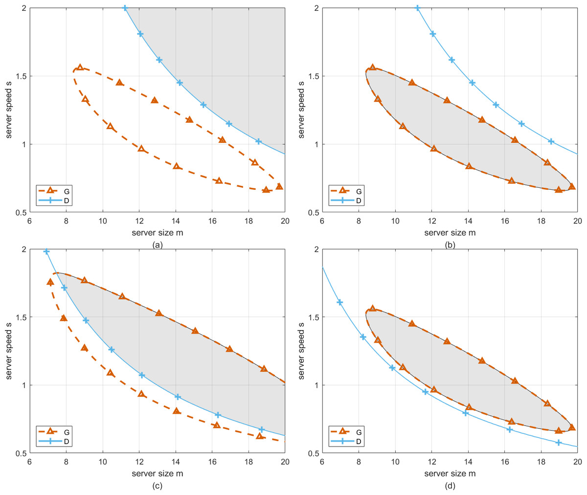
Figure 6: The feasible region related to G and D.
Firstly, two cases in Figs. 6A and 6B are discussed. In these cases, one region has not intersected with the other, namely, the working point selected in each region to configure server size and speed can only satisfy one requirement of cloud service providers or customers. Therefore, we have to take the robustness analysis with respect to the working point in T-feasible region or G-feasible region individually. Correspondingly, the detailed descriptions can be found in ‘Deadline aware configuration’ and ‘Profit aware configuration’ respectively. Secondly, the case in Fig. 6C shows that one region has intersected with the other, and the case in Fig. 6D shows that G-feasible region has been completely covered by T-feasible region. Both of these cases represent the working point selected in the overlapping region to configure server size and speed can satisfy the requirements of cloud service providers or customers simultaneously. Correspondingly, the detailed descriptions can be found in ‘Profit and deadline aware configuration’.
Deadline aware configuration
In this section, the goal is to ensure that customer requests are processed within a specified time-frame. Perturbations in server size and speed can significantly impact the system’s ability to meet these deadlines. For instance, if server size or speed decreases unexpectedly, the waiting time for customers may increase, leading to missed deadlines. Figure 6A illustrates how the T-feasible region, which ensures acceptable waiting time, is affected by changes in server size and speed.
As can be seen from Fig. 6A, the robustness analysis with respect to the working point in T-feasible region rather than G-feasible region is considered. In this case, we merely pursue the optimal configuration of server size and speed that ensure the strongest robustness of the system towards waiting time of customers, which is equivalent to search working point with the longest robustness radius according to Eq. (23) in T-feasible region.
To achieve the optimal configuration of server size and speed in the system, DBO is introduced to perform heuristic searching in T-feasible region. Please note that the fitness of population generated in each iteration is obtained by Algorithm 2 . The pseudo code of DBO algorithm is given in Algorithm 3 .
__________________________________________________________________________________________
  Algorithm 3: Robust configuration method based on DBO algorithm_________
    Input: The maximum iterations tmax, the size of the population N
    Output: Optimal position xz andits radius r
 1  Initialize the population i ← 1,2,...,N; xz ← [mz,sz]; b, k,S,g,e1,e2;
  2  while t < tmax do
     3   for  i ← 1 to N do
    4   if i is ball-rolling dung beetle then
5   δ ← rand(1);
6   if δ < 0.9 then
7   α ←through the α selection strategy;
8   xt+1
i    ← xt
i + αkxt−1
i    + b|xt
i − xt
w|; Obtain the ri of xt+1
i
by Algorithm 1;
9   else
10   θ ←through the θ selection strategy;
xt+1
i    ← xt
i + tanθ∣ ∣
 xti − xt−1
i   ∣ ∣
       ; Obtain the ri of xt+1
i    by
Algorithm 1;
11   end
12   end
13   if i is brood ball then
14   Update boundary selection based on x′
g;
15   Obtain the ri corresponding to xt+1
i    by Algorithm 1;
16   end
17   if i is small dung beetle then
18   xt+1
i    ← xt
i + e1 (
   xti − lb′
          )
        + e2 (
   xti − ub′
          )
         ; Obtain the ri of
xt+1
i    by Algorithm 1;
19   end
20   if i is thief  then
21   xt+1
i    ← xt
l+Sg(|xt
i − xt
g| + |xt
i − xt
l|); Obtain the ri of xt+1
i    by
Algorithm 1;
22   end
23   end
24   if the newly generated r is better than before then
    25   r ← ri; xz ← xt+1
i   ;
26   end
27   t ← t + 1;
28  end
By setting deadline as D = 0.001, and replacing T in Eq. (19) by it, we draw the boundary of T-feasible region, which is shown as the red curve in Fig. 7. As can be seen from Fig. 7, the working point with the longest robustness radius can be found in the upper-right corner with server size and speed equal to 20 and 2, respectively. An intuitive explanation can be given as below. The system with bigger server size and speed owns stronger quality of service, which will certainly lead to a smaller possibility that waiting time of customers exceeds deadline. However, even if the strongest robustness of the system towards waiting time of customers can be obtained, the price that the system has to pay is the minimization in profit of cloud service providers, which is not benefit for the long-term operation of the system. Therefore, the chosen working point [20, 2] in the upper-right corner not only minimizes the risk of exceeding deadlines but also maximizes the system’s resilience to such perturbations. This balance is crucial for maintaining service quality despite the inevitable uncertainties in server performance.
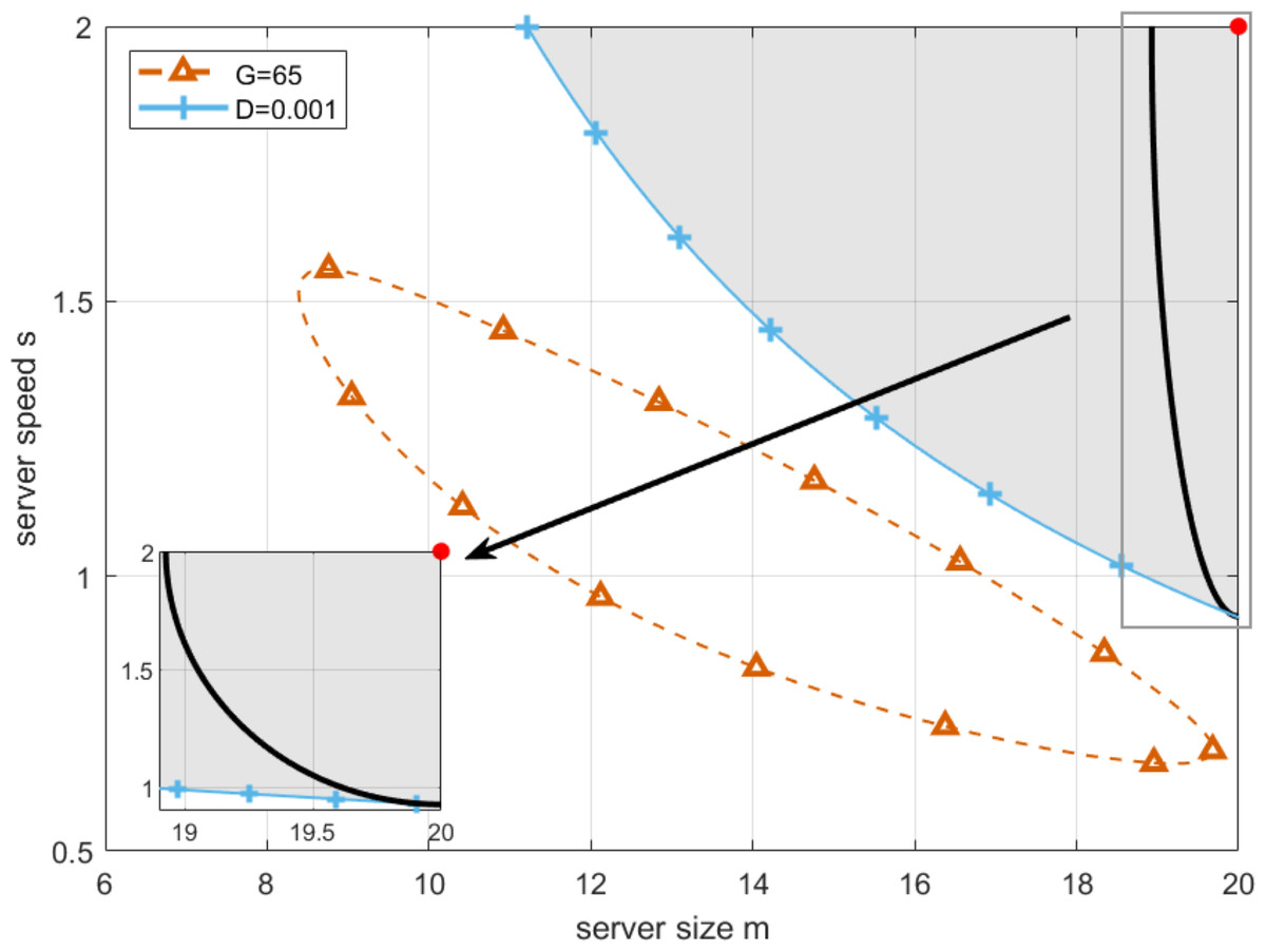
Figure 7: Deadline aware optimal working point.
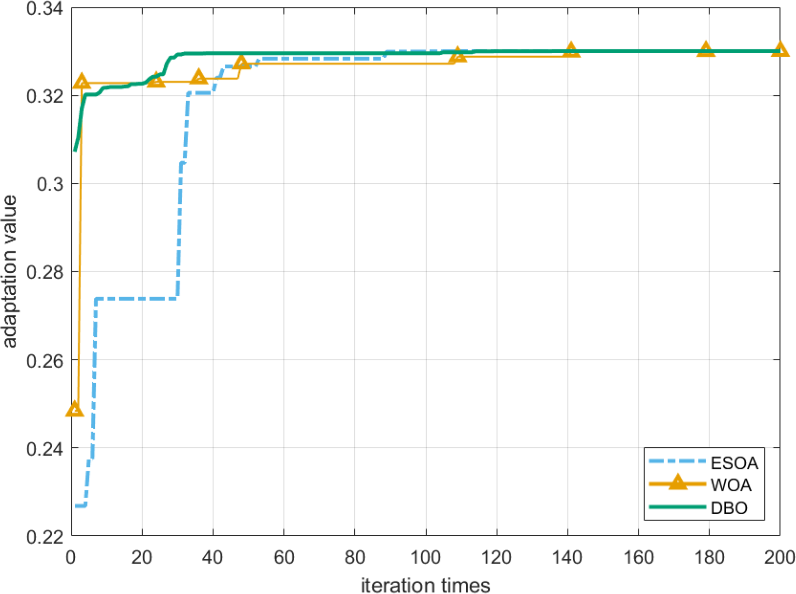
To prove the feasibility of the DBO algorithm, the robustness radius is selected as the fitness function of these heuristic algorithms. It can be seen from Fig. 8 that the DBO algorithm can achieve the global optimum with the least number of iterations. In addition, after 200 iterations, the robust radius obtained by DBO and ESOA algorithms is the same and the longest, while the effect of WOA is inferior to them. We also confirm this conclusion through Tables 2 and 3.
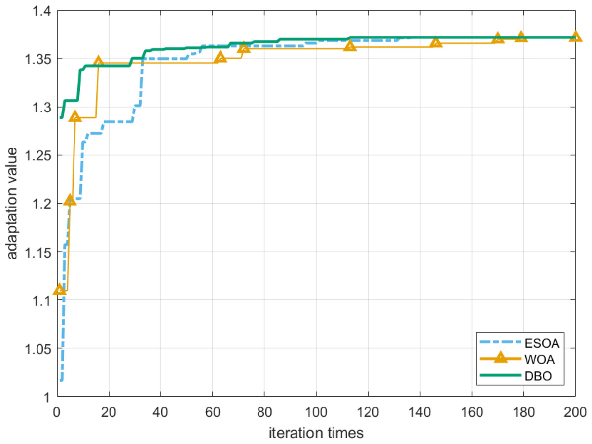
Figure 8: Convergence of robustness radius r.
We perform a robustness analysis of the situation shown in Fig. 6A. At this time, let λ be fixed, and the deadlines are set to D = 0.001, D = 0.1 and D = 1, respectively. It can be found from Fig. 9A that the DBO-based robust configuration method can obtain the Optimal working point at the same location in the three cases where the server size and speed are mz = 20 and sz = 2, respectively. The longest robustness radii are 1.073185, 1.371784, and 1.45464, respectively. The intuitive explanation is as follows. The greater the deadline, the less likely the customer’s waiting time will exceed the deadline. Table 2 shows the results of the DBO algorithm and other comparison algorithms for this analysis.
Through Fig. 9B, we describe how the robustness radius of the system changes with λ at a fixed deadline, where the dotted box represents the T-feasible region of the equivalent change when λ changes. Specifically, when λ increases, the robustness radius increases accordingly. This means that in the case of higher arrival rates, the system needs to be robust on a wider scale to ensure that service requests can be processed promptly within a given deadline. Table 3 provides specific values, showing the change of the robustness radius of the system under different arrival rates. These data further confirm the trend in Fig. 9B. The data in the table provides a quantitative reference for system designers to optimize the configuration in practical applications.
| Parameters | ESOA solution | WOA solution | DBO solution | |||||||
|---|---|---|---|---|---|---|---|---|---|---|
| λ | D | m | s | r | m | s | r | m | s | r |
| 10 | 1 | 20.0000 | 2.0000 | 1.454264 | 19.9580 | 1.9999 | 1.452994 | 20.0000 | 2.0000 | 1.454264 |
| 10 | 0.1 | 20.0000 | 2.0000 | 1.371784 | 19.9884 | 1.9999 | 1.371303 | 20.0000 | 2.0000 | 1.371784 |
| 10 | 0.001 | 20.0000 | 2.0000 | 1.073185 | 19.9998 | 1.9991 | 1.072235 | 20.0000 | 2.0000 | 1.073185 |
| Parameters | ESOA solution | WOA solution | DBO solution | |||||||
|---|---|---|---|---|---|---|---|---|---|---|
| λ | D | m | s | r | m | s | r | m | s | r |
| 10 | 0.1 | 20.0000 | 2.0000 | 1.371784 | 19.9884 | 1.9999 | 1.371303 | 20.0000 | 2.0000 | 1.371784 |
| 12 | 0.1 | 25.0000 | 2.5000 | 1.914081 | 24.9860 | 2.4998 | 1.913531 | 25.0000 | 2.5000 | 1.914081 |
| 14 | 0.1 | 30.0000 | 3.0000 | 2.442344 | 29.9749 | 2.9998 | 2.441594 | 30.0000 | 3.0000 | 2.442344 |
| 16 | 0.1 | 35.0000 | 3.5000 | 2.962600 | 34.9726 | 3.4997 | 2.961919 | 35.0000 | 3.5000 | 2.962600 |
| 18 | 0.1 | 40.0000 | 4.0000 | 3.477881 | 39.9918 | 3.9990 | 3.476800 | 40.0000 | 4.0000 | 3.477881 |
| 20 | 0.1 | 45.0000 | 4.5000 | 3.989867 | 44.9870 | 4.4992 | 3.988864 | 45.0000 | 4.5000 | 3.989867 |
Profit aware configuration
In this section, the primary objective is to maximize the profit of cloud service providers. Perturbations in server size and speed can affect the system’s profitability. For example, a decrease in server speed may lead to increased operational costs or reduced service quality, impacting the overall profit. As shown in Fig. 6B, the G-feasible region represents the configurations that ensure acceptable profit. Perturbations can shift the working point outside this region, leading to suboptimal profit outcomes. In this case, we merely pursue the optimal configuration of server size and speed that ensures the strongest robustness of the system towards the profit of cloud service provider, which is equivalent to search working point with the longest robustness radius according to Eq. (23) in G-feasible region.
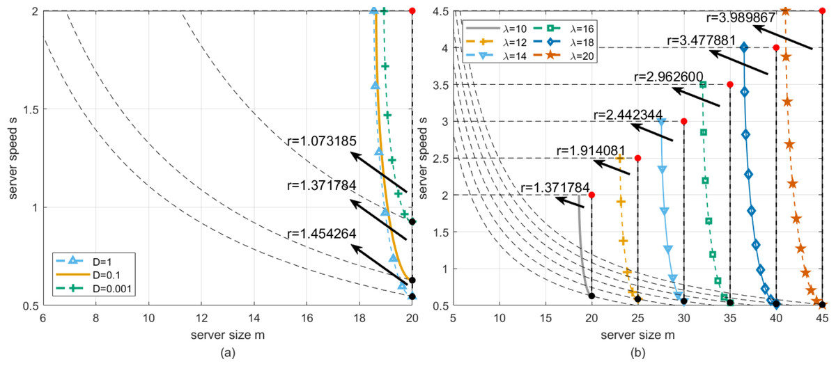
Figure 9: (A) Longest robustness radius rversusD when λ is fixed. (B) Longest robustness radius rversusλ when D is fixed.
As can be seen from Fig. 6B, the robustness analysis with respect to the working point in G-feasible region rather than T-feasible region is considered. In this case, we merely pursue the optimal configuration of server size and speed that ensures the strongest robustness of the system towards the profit of cloud service providers, which is equivalent to searching the working point with the longest robustness radius in G-feasible region.
Now, the optimal configuration of server size and speed can be obtained by the algorithm similar to the one applied in the previous subsection. By setting the lowest profit that cloud service providers can accept as G = 65, and substituting it in Eq. (21), we draw the boundary of G-feasible region, which is shown as the blue curve in Fig. 10. As can be seen from Fig. 10, the working point with the longest robustness radius can be found in the center with server size and speed equal to 12.7981 and 1.1153, respectively. Please note that since the boundary of G-feasible region is closed, the idea of keeping the working point away from the boundary as far as possible applied in the previous subsection is not suitable for the case in this subsection. Therefore, the chosen working point in the center not only meets the profit requirements but also maximizes the system’s resilience to such perturbations. This balance is essential for ensuring both profitability and stability in the face of unavoidable uncertainties in server performance.
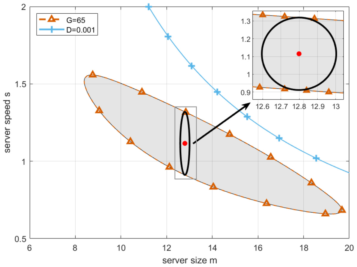
Figure 10: Profit aware optimal working point.
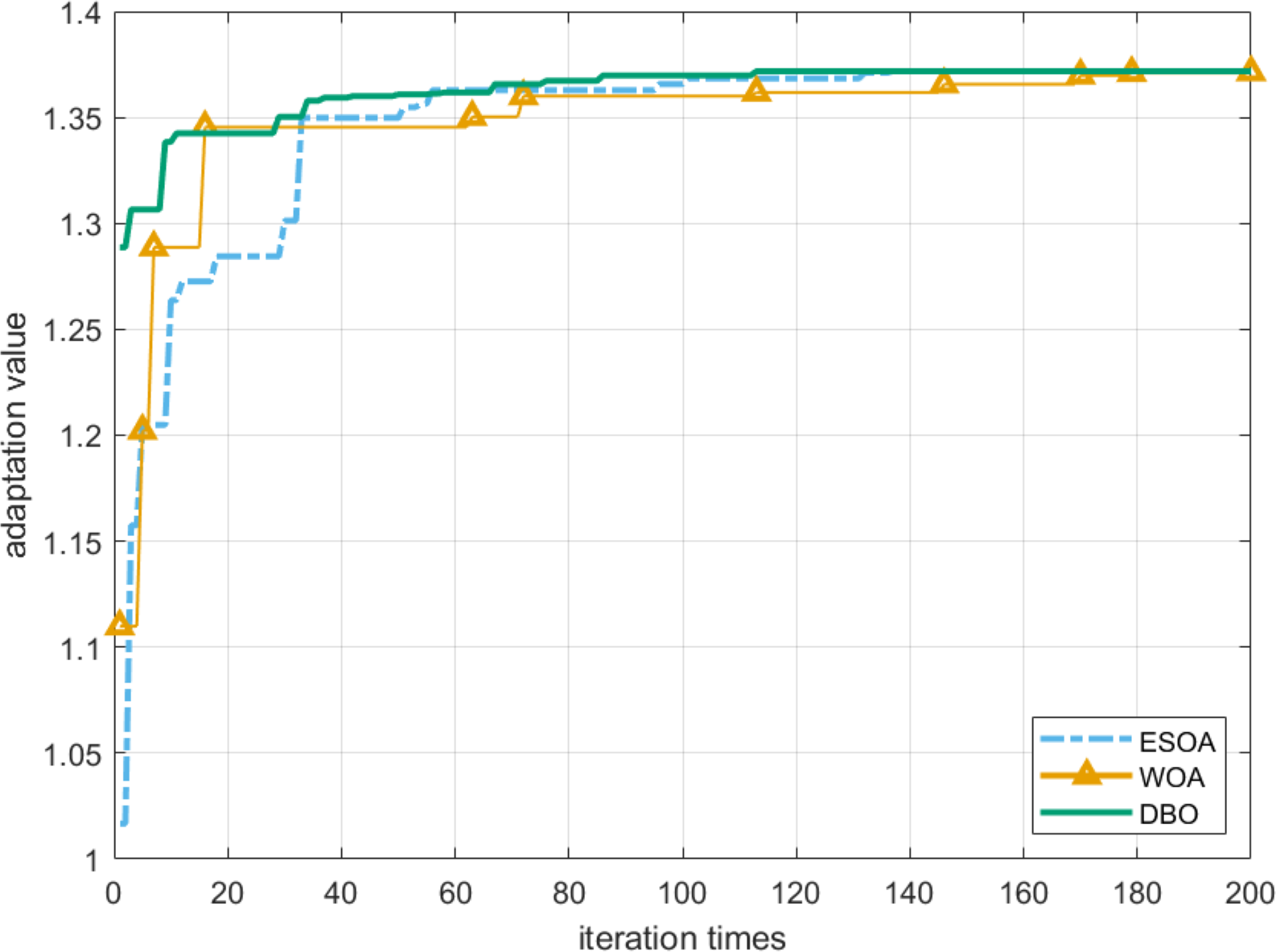
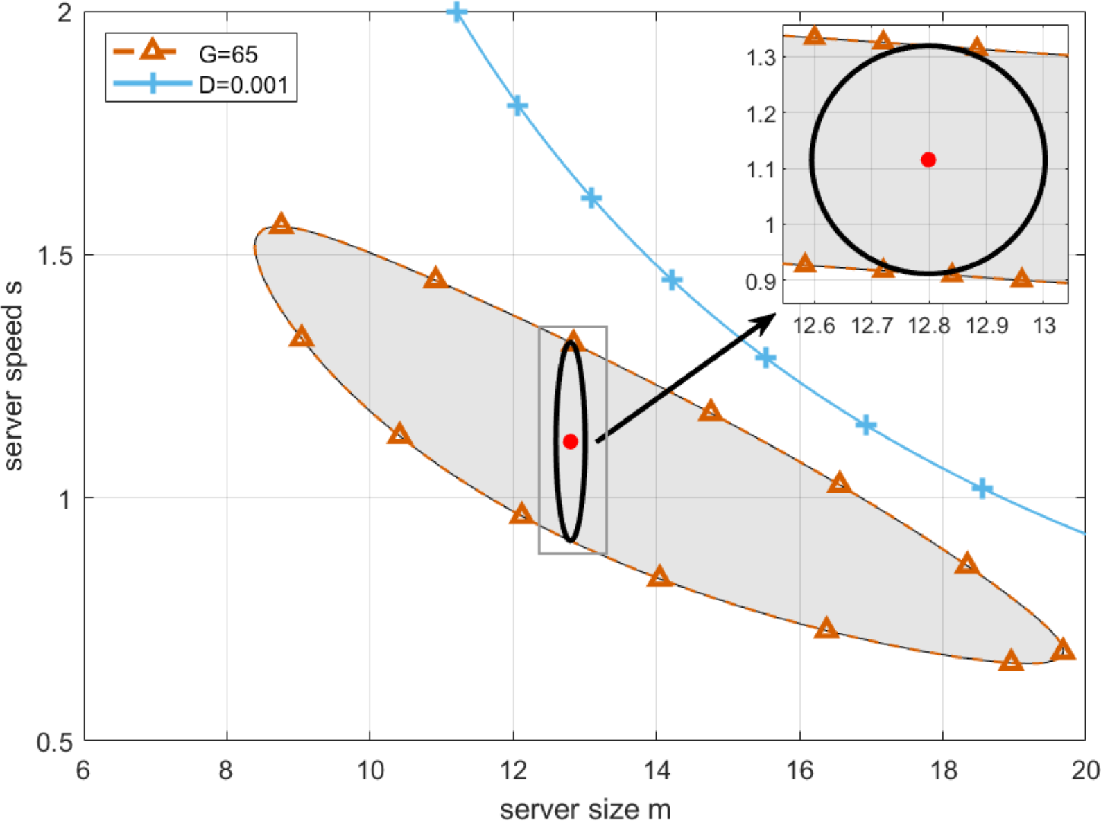
To verify the superiority of the DBO algorithm, ESOA and WOA are adopted to obtain a robustness radius as well. Note that the robustness radius is selected as the fitness function of these heuristic algorithms. It can be seen from Fig. 11 that the longest robust radius obtained by all these algorithms after 200 iterations is basically the same, and the DBO algorithm can achieve the global optimum with the least number of iterations. In addition, we can find from Table 4 that the results obtained by DBO are superior to other comparison algorithms when solving this problem.
Figure 11: Convergence of robustness radius r.
Then, we perform the robustness analysis for the case presented in Fig. 6B with the lowest profit that cloud service providers can accept being set to G = 55, G = 60 and G = 65, respectively. As can be seen from Fig. 12A, by simulating the proposed algorithm, the optimal working point can be obtained for three cases, where server size and speed equal to [13.6891, 1.2479], [13.2120, 1.1846], [12.7987, 1.1153], respectively, and the corresponding longest robustness radii are 0.440086, 0.330031 and 0.203571. Then, for the purpose of practical application, we further find the approximate solution in the neighborhood of the optimal working point. Firstly, by setting server size to the floor of the abscissa of the optimal working point, and adopting Algorithm 2 to obtain the corresponding server speed, we have one group of actual optimal working point with server size and speed equal to [13, 1.2891], [13, 1.1982], [12, 1.1733] for the three cases, and the corresponding robustness radii are 0.438730, 0.329844 and 0.201064. Secondly, by setting server size to the ceiling of the abscissa of the optimal working point, and to obtain the corresponding server speed with the same method, we have another group of actual optimal working point with server size and speed equal to [14, 1.2300], [14, 1.1356], [13, 1.1012] for the three cases, and the corresponding robustness radii are 0.439834, 0.328240 and 0.203329. Finally, to compare the robustness radii for each case, the actual optimal working point with a larger robustness radius is chosen to configure the cloud computing platform.
| Parameters | ESOA solution | WOA solution | DBO solution | |||||||
|---|---|---|---|---|---|---|---|---|---|---|
| λ | G | m | s | r | m | s | r | m | s | r |
| 10 | 55 | 13.8169 | 1.2405 | 0.439986 | 13.8417 | 1.2391 | 0.440028 | 13.6891 | 1.2479 | 0.440086 |
| 10 | 60 | 13.3167 | 1.1779 | 0.330009 | 13.1684 | 1.1873 | 0.330019 | 13.2120 | 1.1846 | 0.330031 |
| 10 | 65 | 12.9005 | 1.1081 | 0.203472 | 12.8649 | 1.1106 | 0.203526 | 12.7987 | 1.1153 | 0.203571 |
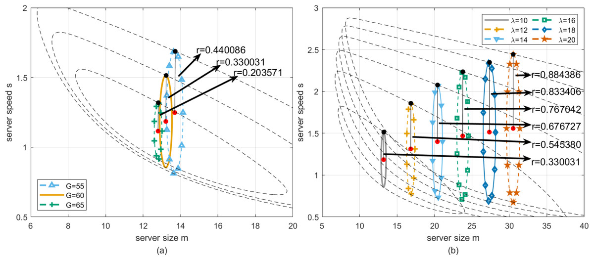
Figure 12: (A) Longest robustness radius rversusG when λ is fixed. (B) Longest robustness radius rversusλ when G is fixed.
Furthermore, we perform the robustness analysis for the case presented in Fig. 6B when the arrival rate of customers changes. In this case, λ is selected in and G remains the same. As can be seen from Fig. 12B, by simulating the proposed algorithm, the optimal working point can be obtained for six cases, where server size and speed equal to [13.2120, 1.1846], [16.8255, 1.3126], [20.3930, 1.3997], [23.1644, 1.4676], [27.3285, 1.5135], [30.5062, 1.5577] respectively, and the corresponding longest robustness radii are 0.330031, 0.545380, 0.676727, 0.767042, 0.833406 and 0.884386. Then, for practical application, we further find the approximate solution in the neighborhood of the optimal working point. Similarly, by setting server size to the floor of the abscissa of the optimal working point, and adopting Algorithm 2 to obtain the corresponding server speed, we have one group of actual optimal working point with server size and speed equal to [13, 1.1982], [16, 1.3507], [20, 1.4137], [23, 1.4902], [27, 1.521646], [30, 1.5688] for the six cases, and the corresponding robustness radii are 0.329844, 0.544136, 0.676582, 0.766546, 0.833346, 0.884203. Secondly, by setting server size to the ceiling of the abscissa of the optimal working point, and to obtain the corresponding server speed with the same method, we have another group of actual optimal working point with server size and speed equal to [14, 1.1356], [17, 1.3048], [21, 1.3786], [24, 1.4607], [28, 1.4970], [31, 1.5470] for the three cases, and the corresponding robustness radii are 0.328240, 0.545326, 0.676336, 0.767023, 0.833110 and 0.884336. Finally, according to the selection principle to maximize the robustness radius, the actual optimal working point that makes the robustness radius larger is determined as a better solution to configure the cloud computing system.
Figure 12B depicts how the robustness radius of the system changes with the arrival rate under fixed profit. Specifically, when the arrival rate increases, the robustness radius increases accordingly. This means that in the case of higher arrival rates, the system needs to be robust in a wider range to ensure that service requests can be effectively processed under given profit requirements.
Table 5 provides specific values, showing the change in the robustness radius of the system under different arrival rates. These data further confirm the trend in Fig. 12B: as the arrival rate increases, the robustness radius increases. The data in the table provides a quantitative reference for system designers to optimize the configuration in practical applications to ensure the robustness and profitability of the system under various load conditions.
| Parameters | ESOA solution | WOA solution | DBO solution | |||||||
|---|---|---|---|---|---|---|---|---|---|---|
| λ | G | m | s | r | m | s | r | m | s | r |
| 10 | 60 | 13.1684 | 1.1873 | 0.330019 | 13.3167 | 1.1779 | 0.330009 | 13.2120 | 1.1846 | 0.330031 |
| 12 | 60 | 16.7940 | 1.3140 | 0.545375 | 16.7911 | 1.3142 | 0.545320 | 16.8255 | 1.3126 | 0.545380 |
| 14 | 60 | 20.3945 | 1.3997 | 0.676726 | 20.4068 | 1.3993 | 0.676722 | 20.3930 | 1.3997 | 0.676727 |
| 16 | 60 | 23.8966 | 1.4637 | 0.767042 | 23.8270 | 1.4657 | 0.767003 | 23.1644 | 1.4676 | 0.767042 |
| 18 | 60 | 27.6793 | 1.5048 | 0.833319 | 27.0071 | 1.5215 | 0.833363 | 27.3285 | 1.5135 | 0.833406 |
| 20 | 60 | 30.6645 | 1.5542 | 0.884398 | 30.5564 | 1.5666 | 0.884365 | 30.5062 | 1.5577 | 0.884386 |
Profit and deadline aware configuration
By summarizing the previous discussions about robustness analysis, the maximization problems of robustness radius with respect to the working point in T-feasible region and G-feasible region are discussed separately. However, when referring to the requirements of cloud service providers and customers, one to be satisfied always comes with the cost of impairing another. Therefore, it is necessary to find the optimal working point by combining with T-feasible region and G-feasible region.
Now, the cases presented in Figs. 6C and 6D are taken into consideration. Please note that the case presented in Fig. 6D is similar to the one in Fig. 6B, the only difference is that the optimal working point selected in the former case satisfies the requirement of customers as well, while the one chosen in the latter case is not. In this subsection, we mainly focus on the case presented in Fig. 6C.
By setting deadline as D = 0.1, and replacing T in Eq. (19) by it, setting the lowest profit that cloud service providers can accept as G = 60, and substituting it in Eq. (21), we draw the boundaries of T-feasible region and G-feasible region, which are shown as the red and blue curve in Fig. 13 respectively.
(26)where, G denotes the lowest profit that cloud service providers can accept, and D denotes the deadline. To solve the multi-objective programming model presented in Eq. (26), Non-dominated Sorting Genetic Algorithms II (NSGA-II) is introduced in this article. The pseudo code for such algorithm is shown in Algorithm 4 .
__________________________________________________________________________________________
  Algorithm 4: Robust configuration based on NSGA-II algorithm     _________
    Input:  interval of server size[mmin,mmax], server speed[smin,smax]
    Output: optimal h1,h2
  1  begin
     2   t ← 1,i ← 1;
3   Initialize the population in the given interval;
4   The fitness value Y is calculated through Algorithm 1;
5   T1 ← perform non-dominated sorting strategy;
6   Sort f by crowding distance for each rank ;
7   while t < Max number of iterations do
    8   Pt ← create parent by T1 using tournament selected;
9   Qt ← create offspring by Pt using selection, crossover and
mutation;
10   Rt ← Pt ∪ Qt ;
11   The fitness value Yt is calculated through Algorithm 1;
12   Ft ← calculate all non-dominated fronts of Rt;
13   Pt+1 ←∅ ;
14   while |Pt+1|∪∣ ∣
 Fit∣ ∣
   ≤ N do
15   Fit ← select ith non-dominated front in Ft using crowding
distance sorting strategy;
16   Pt ← Pt+1 ∪ Fit;
17   i ← i + 1;
18   end
19   Tt+1 ← Pt+1 ∪ Ft [1 : (N −|Pt+1|)];
20   t ← t + 1;
21   end
22 end 
Figure 13: Profit and deadline aware optimal working point.
By applying Algorithm 4 in Eq. (26), the result can be shown in Fig. 13. As can be seen from Fig. 14, each point on the Pareto frontier represents an optimal solution for the multi-objective programming model. Without loss of generality, we choose the red point marked in Fig. 14 as the best point on the left side as the optimal working point. On this basis, by setting server size and speed to mz = 14.5967 and sz = 1.1518, we can obtain the first fitness function as and the second fitness function as r1 + r2 = 0.5419. In this case, the longest robustness radius from the working point to the boundaries of T-feasible region and G-feasible region are r1 = 0.2709 and r2 = 0.2709 respectively. Then, for practical application, we further find the approximate solution in the neighborhood of the optimal working point. By setting server size to the floor and ceiling of the abscissa of the optimal working point, and adopting Algorithm 4 to obtain the corresponding server speed, we have the actual optimal working point with server size and speed equal to [14, 1.1922] and [15, 1.1260], respectively. Moreover, since the robustness radius corresponding to the two cases are 0.270 and 0.268, respectively, the actual optimal working point with a larger robustness radius is chosen to configure the cloud computing platform.
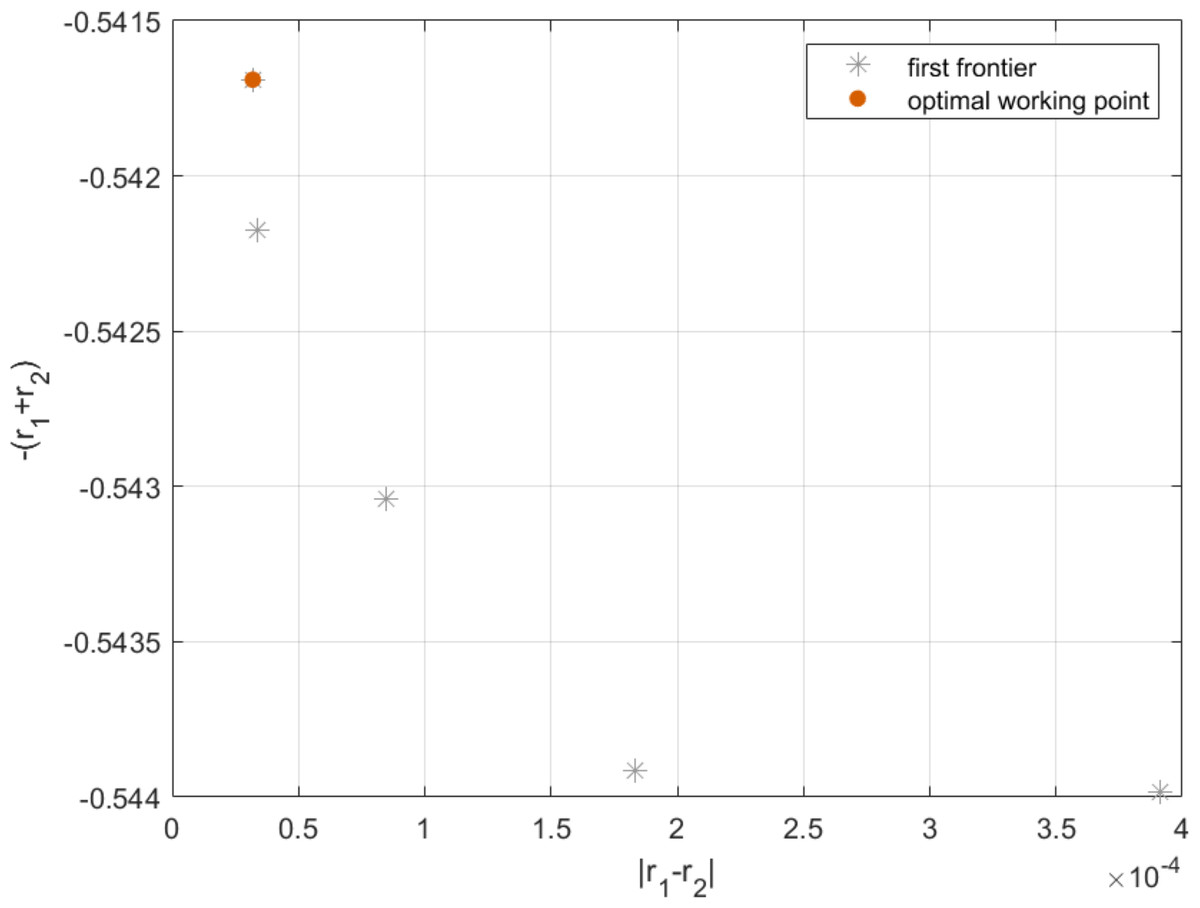
Figure 14: Pareto frontier of h1 and h2 .
Results
In order to make our scheme more reliable, we further discuss the results obtained from the above experiments.
When only considering customer demands, we analyze the results obtained by the robust configuration method in the case of deadline changes (i.e., Fig. 9A) and arrival rate changes (i.e., Fig. 9B) in more detail. In order to verify the accuracy of the obtained results, we compare our scheme with the brute force search (BFS) method (Suzuki et al., 2021) through the verification method of literature (Cong et al., 2022), which can find the optimal solution in the T-feasible region. Table 6 compares our solution with the solution obtained by BFS at different deadlines. Table 7 compares our solution with the solution obtained by BFS at different λ. Referring to these tables, we can find that for this problem, our scheme is consistent with the value of the solution obtained by BFS.
Similarly, when only the needs of cloud service providers are considered, we also analyze in more detail the results obtained by the robust configuration method in the case of lowest profit changes (i.e., Fig. 12A) and arrival rate changes (i.e., Fig. 12B). To verify the efficacy of our scheme, we compare our scheme with BFS. Table 8 compares our solution with the solution obtained by BFS at different lowest profit. Table 9 compares our scheme with the solution obtained by BFS under different λ. In the simulation, BFS iterates 40 billion times for each set of parameters. As can be seen the magnitude error of the solution obtained by our scheme and BFS is on the order of 10−6, indicating that our solution is very close to the optimal solution.
| Parameters | BFS solution | DBO solution | Opt_Dev | |||||
|---|---|---|---|---|---|---|---|---|
| λ | T | mBFS | sBFS | rBFS | mDBO | sDBO | rDBO | |
| 10 | 1 | 20.0000 | 2.0000 | 1.45426478 | 20.0000 | 2.0000 | 1.45426478 | 0.000000% |
| 10 | 0.1 | 20.0000 | 2.0000 | 1.37178428 | 20.0000 | 2.0000 | 1.37178428 | 0.000000% |
| 10 | 0.001 | 20.0000 | 2.0000 | 1.07318541 | 20.0000 | 2.0000 | 1.07318541 | 0.000000% |
| Parameters | BFS solution | DBO solution | Opt_Dev | |||||
|---|---|---|---|---|---|---|---|---|
| λ | T | mBFS | sBFS | rBFS | mDBO | sDBO | rDBO | |
| 10 | 0.1 | 20.0000 | 2.0000 | 1.37178428 | 20.0000 | 2.0000 | 1.37178428 | 0.000000% |
| 12 | 0.1 | 25.0000 | 2.5000 | 1.91408138 | 25.0000 | 2.5000 | 1.91408138 | 0.000000% |
| 14 | 0.1 | 30.0000 | 3.0000 | 2.44234351 | 30.0000 | 3.0000 | 2.44234351 | 0.000000% |
| 16 | 0.1 | 35.0000 | 3.5000 | 2.96259983 | 35.0000 | 3.5000 | 2.96259983 | 0.000000% |
| 18 | 0.1 | 40.0000 | 4.0000 | 3.47788146 | 40.0000 | 4.0000 | 3.47788146 | 0.000000% |
| 20 | 0.1 | 45.0000 | 4.5000 | 3.98986718 | 45.0000 | 4.5000 | 3.98986718 | 0.000000% |
| Parameters | BFS solution | DBO solution | Opt_Dev | |||||
|---|---|---|---|---|---|---|---|---|
| λ | G | mBFS | sBFS | rBFS | mDBO | sDBO | rDBO | |
| 10 | 55 | 13.6934 | 1.2477 | 0.44008631 | 13.6891 | 1.2479 | 0.44008625 | 0.000013% |
| 10 | 60 | 13.2191 | 1.1841 | 0.33003176 | 13.2120 | 1.1846 | 0.33003117 | 0.000178% |
| 10 | 65 | 12.7898 | 1.1159 | 0.20357182 | 12.7987 | 1.1153 | 0.20357106 | 0.000370% |
| Parameters | BFS solution | DBO solution | Opt_Dev | |||||
|---|---|---|---|---|---|---|---|---|
| λ | G | mBFS | sBFS | rBFS | mDBO | sDBO | rDBO | |
| 10 | 60 | 13.2191 | 1.1841 | 0.33003176 | 13.2120 | 1.1846 | 0.33003117 | 0.000178% |
| 12 | 60 | 16.8257 | 1.3126 | 0.54537972 | 16.8255 | 1.3126 | 0.54537966 | 0.000010% |
| 14 | 60 | 20.3925 | 1.3998 | 0.67672704 | 20.3930 | 1.3997 | 0.67672701 | 0.000004% |
| 16 | 60 | 23.8241 | 1.4658 | 0.76704506 | 23.7644 | 1.4676 | 0.76704205 | 0.000392% |
| 18 | 60 | 27.2783 | 1.5147 | 0.83340771 | 27.3285 | 1.5135 | 0.83340562 | 0.000250% |
| 20 | 60 | 30.6662 | 1.5542 | 0.88438818 | 30.5062 | 1.5577 | 0.88438644 | 0.000197% |
Experiments show that the proposed method is effective in determining robustness configurations that can consistently find the optimal working point within the feasible region of acceptable performance degradation, i.e., maintaining the system performance at an acceptable level in the presence of perturbations.
Discussion
Our research addresses dealing with the impact of unforeseen perturbations (such as server failure, bandwidth sharing, voltage fluctuations, etc.) on system performance in cloud computing environments and proposes a robust configuration strategy. This strategy not only focuses on the optimization of profit and waiting time but more importantly, proposes a method to maintain the minimum bottom line of system performance under perturbation. This differs from the previous research in the pursuit of profit maximization and waiting time minimization, which reflects the originality of our research.
Moreover, we confirm the consistent performance of the proposed robust configuration strategy under various perturbation conditions through repeated experiments in different environments. This verification can not only help to improve the reliability and applicability of the scheme and make it more convincing in practical applications but also provide practical guidance for cloud service providers to deal with perturbations in practical applications.
In addition, the research on this kind of robustness problem is also widely used in real life. For example, in order to ensure the stability and high availability of services, Netflix, one of the world’s largest streaming media service providers, adopts a hybrid cloud strategy and uses robust optimization methods to deal with unpredictable traffic fluctuations and failures. Google’s Spanner uses a variety of robust optimization techniques to ensure its stability in the face of unpredictable events such as network partitions and server failures. To improve the robustness of the system, the global mobility platform Uber uses a variety of optimization algorithms to dynamically adjust pricing and resource allocation.
Therefore, our proposed robust configuration scheme offers significant benefits for cloud service providers and customers. For providers, the scheme ensures that the system can maintain acceptable profit levels even under severe perturbations. For customers, it guarantees that the waiting time remains within acceptable bounds, thereby enhancing their satisfaction.
Although the methods proposed in this study perform effectively in many aspects, there are still some limitations. First of all, this study focuses on the problem of resource allocation in a single cloud environment, and does not involve more complex parallel systems. In practical applications, cloud computing usually involves multiple data centers and complex parallel task scheduling. Extending the method of this study to these more complex environments will be a direction worth exploring. Additionally, this study assumes that the perturbation is predictable and quantifiable. However, in practical applications, the source and nature of perturbations may be more complex and difficult to predict. Therefore, more advanced perturbation prediction and modeling techniques can be considered in future research to improve the accuracy and applicability of robust configuration. In addition, although the heuristic optimization algorithm in this study performs well in experiments, it may face computational efficiency problems when dealing with large-scale cloud environments. Future research can consider introducing more efficient algorithms, such as machine learning-based methods, to improve computational efficiency in large-scale environments.
By addressing these limitations and exploring new research directions, research on the robustness of cloud computing resource allocation will be able to better cope with complex and dynamic practical requirements and further improve the reliability and performance of cloud services.
Conclusion
The novelty of this study is that it focuses on robustness under unpredictable perturbations, which is a key but often overlooked aspect of cloud computing. Therefore, we propose a robust configuration strategy in the cloud computing environment using a heuristic optimization algorithm. The main purpose is to mitigate the negative impact of unpredictable perturbations on system performance and ensure that cloud service providers and customers achieve their desired results. In this article, we define the bottom line as an acceptable feasible region by establishing the profit and waiting time that cloud service providers and customers care about as performance indicators. Several possible simulation experiments are designed to create a cloud environment with perturbations. This provides a realistic context for the subsequent analysis, so that the results have practical significance. Then, by defining the shortest distance from the working point to the performance baseline to measure the robustness of the system, the performance of the system under perturbation conditions is comprehensively evaluated.
Finally, by using our proposed method, we find the optimal configuration on a specific cloud workbench considering different specific perturbations.
Meanwhile, a variety of optimization algorithms and introduced for comparison, and the result reflects the efficiency of our proposed method. By changing the arrival rate or performance indicators of a variety of conditions of verification, to address its limitation. In addition, the error of the solution of our algorithm compared with the most advanced benchmark scheme is on the order of 10−6, indicating the accuracy of our solution.
Through multiple sets of comparative experiments, this study verifies the hypothesis that by optimizing the allocation of cloud computing resources, the profit of cloud service providers can be maximized and the waiting time of customers can be minimized in the presence of perturbations. Our performance-aware robust configuration strategy not only provides a deep understanding of system behavior in theory, but also demonstrates its effectiveness in practice. Through the application in the actual environment, we can significantly improve the robustness of the system and reduce the performance fluctuation caused by unpredictable factors.
The implication of this strategy is that it provides a new perspective for cloud computing resource management, enabling cloud service providers to manage their resources more flexibly and effectively in the face of complex and dynamic service requirements. This not only improves the overall quality of cloud services but also provides a solid foundation for future research and application.