
The k conditional nearest neighbor algorithm for classification and class probability estimation
- Published
- Accepted
- Received
- Academic Editor
- Ciro Cattuto
- Subject Areas
- Data Mining and Machine Learning, Data Science
- Keywords
- Nonparametric classification, Nearest neighbor, Probabilistic classifier
- Copyright
- © 2019 Gweon et al.
- Licence
- This is an open access article distributed under the terms of the Creative Commons Attribution License, which permits unrestricted use, distribution, reproduction and adaptation in any medium and for any purpose provided that it is properly attributed. For attribution, the original author(s), title, publication source (PeerJ Computer Science) and either DOI or URL of the article must be cited.
- Cite this article
- 2019. The k conditional nearest neighbor algorithm for classification and class probability estimation. PeerJ Computer Science 5:e194 https://doi.org/10.7717/peerj-cs.194
Abstract
The k nearest neighbor (kNN) approach is a simple and effective nonparametric algorithm for classification. One of the drawbacks of kNN is that the method can only give coarse estimates of class probabilities, particularly for low values of k. To avoid this drawback, we propose a new nonparametric classification method based on nearest neighbors conditional on each class: the proposed approach calculates the distance between a new instance and the kth nearest neighbor from each class, estimates posterior probabilities of class memberships using the distances, and assigns the instance to the class with the largest posterior. We prove that the proposed approach converges to the Bayes classifier as the size of the training data increases. Further, we extend the proposed approach to an ensemble method. Experiments on benchmark data sets show that both the proposed approach and the ensemble version of the proposed approach on average outperform kNN, weighted kNN, probabilistic kNN and two similar algorithms (LMkNN and MLM-kHNN) in terms of the error rate. A simulation shows that kCNN may be useful for estimating posterior probabilities when the class distributions overlap.
Introduction
Supervised classification is a fundamental problem in supervised learning. A common approach to classification is to assume a distribution for each different class. Nonparametric classifiers are often used when it is difficult to make assumptions about the class distribution for the problem. The k-nearest neighbor (kNN) approach (Fix & Hodges, 1951) is one of the most popular nonparametric approaches (Wu et al., 2008). For an input x, the kNN algorithm identifies k objects in the training data that are closest to x with a predefined metric and makes a prediction by majority vote from the classes of the k objects. Although the kNN method is simple and does not require a priori knowledge about the class distributions, kNN has been successfully applied in many problems such as character recognition (Belongie, Malik & Puzicha, 2002) and image processing (Mensink et al., 2013). A number of experiments on different classification problems have demonstrated its competitive performance (Ripley, 2007). A detailed survey of the literature about kNN can be found in (Bhatia & Vandana, 2010).
One of the drawbacks of kNN is that the method can only give coarse estimates of class probabilities particularly for low values of k. For example, with two neighbours or k = 2 the estimated probabilities can only take the values 0%, 50% or 100% depending on whether 0, 1 or 2 neighbors belong to the class. A probabilistic kNN method (PNN) was proposed in (Holmes & Adams, 2002) for continuous probability estimates. However, PNN and kNN are comparable in terms of classification accuracy, and PNN has greater computational costs than kNN (Manocha & Girolami, 2007).
Many other extensions of kNN have been proposed to improve prediction of classification. One direction is to assign different weights to the k nearest neighbors based on their distances to the input x. Higher weights are given to neighbors with lower distances. Examples include weighted kNN (WkNN) (Dudani, 1976) and fuzzy kNN (Keller, Gray & Givens, 1985). Another approach to improve the prediction of kNN is to use the class local means. One of the successful extensions is the local mean based k nearest neighbor approach (LMkNN) (Mitani & Hamamoto, 2006). For a new test instance x, LMkNN finds the k nearest neighbors in each class and calculates the local mean vector of the k nearest neighbors. The distance between x and each local mean is calculated and the class corresponding to the smallest distance is assigned to x. Empirical evidence suggests that compared to kNN, LMkNN is robust to outliers when the training data are small (Mitani & Hamamoto, 2006). The idea of LMkNN has been applied to many other methods such as pseudo nearest neighbor (Zeng, Yang & Zhao, 2009), group-based classification (Samsudin & Bradley, 2010) and local mean-based pseudo k-nearest neighbor (Gou et al., 2014). Recently, an extension of LMkNN, the multi-local means-based k-harmonic nearest neighbor (MLM-kHNN) (Pan, Wang & Ku, 2017), was introduced. Unlike LMkNN, MLM-kHNN computes k different local mean vectors in each class. MLM-kHNN calculates their harmonic mean distance to x and assigns the class with the minimum distance. An experimental study showed that MLM-kHNN achieves high classification accuracy and is less sensitive to the parameter k, compared to other kNN-based methods. However, those local mean based approaches only produce scores for classification and thus are not appropriate when class probabilities are desired.
In this paper, we propose a new nonparametric classifier, k conditional nearest neighbor (kCNN), based on nearest neighbors conditional on each class. For any positive integer k, the proposed method estimates posterior probabilities using only the kth nearest neighbor in each class. This approach produces continuous class probability estimates at any value of k and thus is advantageous over kNN when posterior probability estimations are required. We show that classification based on those posteriors is approximately Bayes optimal for a two-class problem. Furthermore, we demonstrate that the classification approach converges in probability to the Bayes classifier as the size of the training data increases. We also introduce an ensemble of kCNN (EkCNN) that combines kCNN classifiers with different values for k. Our experiments on benchmark data sets show that the proposed methods perform, on average, better than kNN, WkNN, LMkNN and MLM-kHNN in terms of the error rate. Further analysis also shows that the proposed method is especially advantageous when (i) accurate class probabilities are required, and (ii) class distributions overlap. An application using text data shows that the proposed method may outperform kNN for semi-automated classification.
The algorithm proposed in this paper is meant for situations in which nearest neighbor-type algorithms are attractive, i.e., for highly nonlinear functions where the training data and the number of features are not too large. Other approaches such as Support Vector Machines (Vapnik, 2000) and Random Forest (Breiman & Schapire, 2001) are therefore not considered.
The rest of this paper is organized as follows: in ‘Methods’, we present the details of the proposed method. In ‘Experimental Evaluation’ , we report on experiments that compare the proposed method with other algorithms using benchmark data sets. In ‘Exploring Properties of the Proposed Method’ simulation, we investigate how the decision boundary and probability field of the proposed method vary using simulation data. In ‘Application: semi-automated classification using the Patient Joe text data’, we apply the proposed method to semi-automated classification using “Patient Joe” text data. In ‘Discussion’, we discuss the results. In ‘Conclusion’, we draw conclusions.
Methods
K conditional nearest neighbor
In multi-class classification, an instance with a feature vector x ∈ ℝq is associated with one of the possible classes c1, …, cL. We assume a set of training data containing N classified instances. For any x and a given k, we denote by xk|i the kth nearest neighbor of class ci (i = 1, …, L). Let d(x, xk|i) = |x − xk|i| be the (Euclidean) distance between x and xk|i. Figure 1 illustrates this showing the distance between x and the second nearest neighbor (i.e., k = 2) of each class.

Figure 1: An illustrative example of d(x, xk|i), i = 1,2, when k = 2.
Since the distance for class c1 is smaller, for the given query class c1 has a larger posterior probability than c2.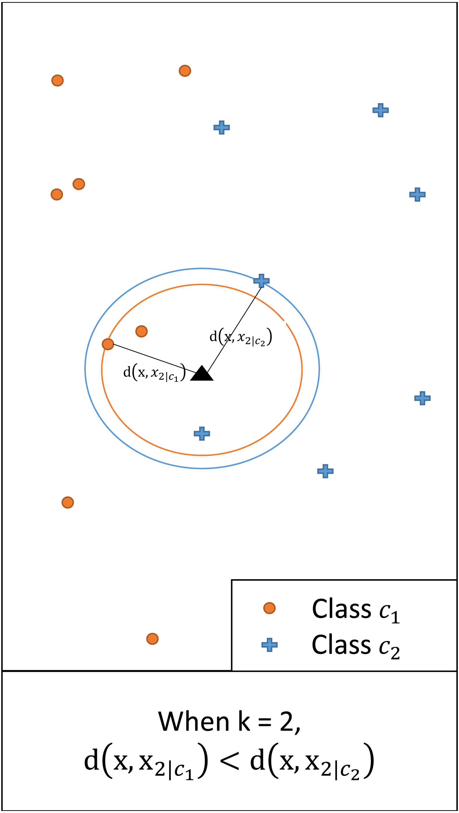
Consider a hypersphere with radius d(x, xk|i) centered at x. By the definition of xk|i, the hypersphere contains k instances of class ci. We may approximate the local conditional density f(x|ci) as (1) where Vk|i is the volume of a hypersphere with radius d(x, xk|i) centered at x and Ni represents the number of instances classified as class ci. This approximation was also introduced in Fukunaga & Hostetler (1975). The approximation assumes that f(x|ci) is nearly constant within the hypersphere of volume Vk|i when the radius d(x, xk|i) is small. Using the prior where and Bayes theorem, the approximate posterior may be obtained as (2) Because , we have . Then, may be obtained as (3) since Vk|i ∝ d(x, xk|i)q. The class with the shortest distance among the L distances has the highest posterior.
The results in Eq. (3) are affected by the dimension of the feature space (q); the class probabilities converge to binary output (1 if the distance is smallest and 0 otherwise) as q increases. This implies the estimated class probabilities will be extreme in high-dimensional data, which is not desirable especially when the confidence of a prediction is required. Since smoothing parameters can improve predictive probability accuracy (e.g., LaPlace smoothing for the Naive Bayes algorithm (Mitchell, 1997), we introduce an optional tuning parameter r as follows: (4) where r ≥ 1 controls the influence of the dimension of the feature space q. As r increases, each posterior converges to 1∕L. That is, increasing r smoothes the posterior estimates.
The k conditional nearest neighbor (kCNN) approach classifies x into the class with the largest estimated posterior probability. That is, class is assigned to x if The proposed classifier is equivalent to kNN when k = 1. We summarize the kCNN classifier in Algorithm 1.
Note that r affects the class probabilities but not the classification. We will show in ‘Ensemble of kCNN’ that the tuning parameter affects the classification of the ensemble of kCNN, which is presented in ‘Ensemble of kCNN’.
_________________________________________________________________________________________________
 Algorithm 1: The k conditional nearest neighbor algorithm
_________________________________________________________________________________________________
      Input: A training data set D, a new instance vector x with dimension q, a positive inte
      ger k, parameter r, a distance metric d
      for i = 1 to L do
         (a) From D, select xk|i, the kth nearest neighbor of x for class ci
         (b) Calculate d(x,xk|i), the distance between x and xk|i
      end for
      for i = 1 to L do
        Obtain ˆ pk(ci|x) ←  d(x,xk|i)−q∕r ____∑Lj=1 d(x,xk|j)−q∕r
      end for
      Classify x into ˆ c if ˆ c = argmax i ˆ pk(ci|x)
__________________________________________________________________________________________________
Figure 2 illustrates an example of a two-class classification problem. For a given k, the method calculates the distance between x and the kth nearest neighbor of each class. When k = 1 and k = 3, class c2 has a larger posterior probability than c1 as the corresponding distance is shorter. When k = 2, however, the posterior probability for class c1 is greater.
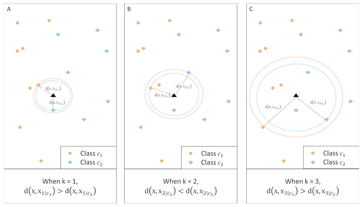
Figure 2: Illustration of kCNN at different values of k.
For any given k, class with a shorter distance has a larger class probability.
Convergence of kCNN
The following theorem says that as the training data increase, kCNN converges to the optimal classifier, the Bayes classifier.
Theorem (convergence of kCNN): Consider a two-class problem with c1 and c2 where p(c1) > 0 and p(c2) > 0. Assume that f(x|ci) (i = 1, 2) is continuous on ℝq. If the following conditions (a) k → ∞, and (b) are satisfied, then for any x where f(x) > 0, kCNN with r = 1 converges in probability to the Bayes classifier.
Proof: Since kCNN makes predictions by approximate posteriors in Eq. (2), it is sufficient to show that converges in probability to the true posterior.
We first consider the convergence of the prior estimate . Let c(j) be the class of the jth training instance. The prior estimate may be described as where I is the indicator function. Hence, by the weak law of large numbers, 1 p(ci).
We next show that the approximation in equation Eq. (1) converges in probability to the true conditional density function. Let be an estimate of the density function f(x) where V is the volume of the hypersphere centered at x containing k training instances. In Loftsgaarden & Quesenberry (1965), it is showed that fN(x) converges in probability to f(x) if k → ∞ and as N increases. We may apply this result to the convergence of the conditional density functions. By the second condition, both and converge to zero. Hence, converges in probability to the true conditional density function f(x|ci).
Since and , Hence, the approximate posterior in Eq. (2) converges in probability to the true posterior. This implies that kCNN converges in probability to the Bayes classifier. ■
The theorem implies that a choice of k needs to be subject to conditions (a) and (b) as the size of the data increases.
Time complexity of kCNN
The time complexity of kNN is O(Nq + Nk) (Zuo, Zhang & Wang, 2008) (O(Nq) for computing distances and O(Nk) for finding the k nearest neighbors and completing the classification). In the classification stage, kCNN (a) calculates the distances between the test instance to all training instances from each class, (b) identifies the kth nearest neighbor from each class, and (c) calculates posterior estimates by comparing the L distances and assigns the test instance to the class with the highest posterior estimate. Step (a) requires O(N1q + ... + NLq) = O(Nq) multiplications. Step (b) requires O(N1k + ... + NLk) = O(Nk) comparisons. Step (c) requires O(L) sum and comparison operations. Therefore, the time complexity for kCNN is O(Nq + Nk + L). In practice, the O(L) component is dominated by the other components, since L is usually much smaller than N. That is, the difference in the complexities between kNN and kCNN is small.
Ensemble of kCNN
The illustrative example in Fig. 2 shows that the classification is affected by the choice of k. Therefore, we propose an ensemble version of kCNN that combines the multiple kCNN algorithms with different values of k. Ensembles are well known as a method for improving predictive performance (Wu et al., 2008; Rokach, 2010). The ensemble of k conditional nearest neighbor (EkCNN) method makes a prediction based on the averaged posteriors for different values of k. These values are now indexed by w: w = 1, …, k. In the ensemble EkCNN, k represents the number of ensemble members. Suppose that posterior probability is estimated by Eq. (4) for each w = 1, …, k. For a new instance x, the predicted class is determined by That is, EkCNN assigns x to the class with the highest average posterior estimate. Unlike kCNN that ignores the first k − 1 nearest neighbors of each class, EkCNN takes into consideration all k distances of each class. Using multiple values of k makes the prediction less reliant on a single k. This may improve the prediction result when the estimated class probabilities are highly variable as a function of k. An illustrative example in Fig. 3 shows that kCNN predicts either point A or point B incorrectly depending on the choice k = 1 or k = 2. However, EkCNN for k = 2 successfully predicts both A and B.
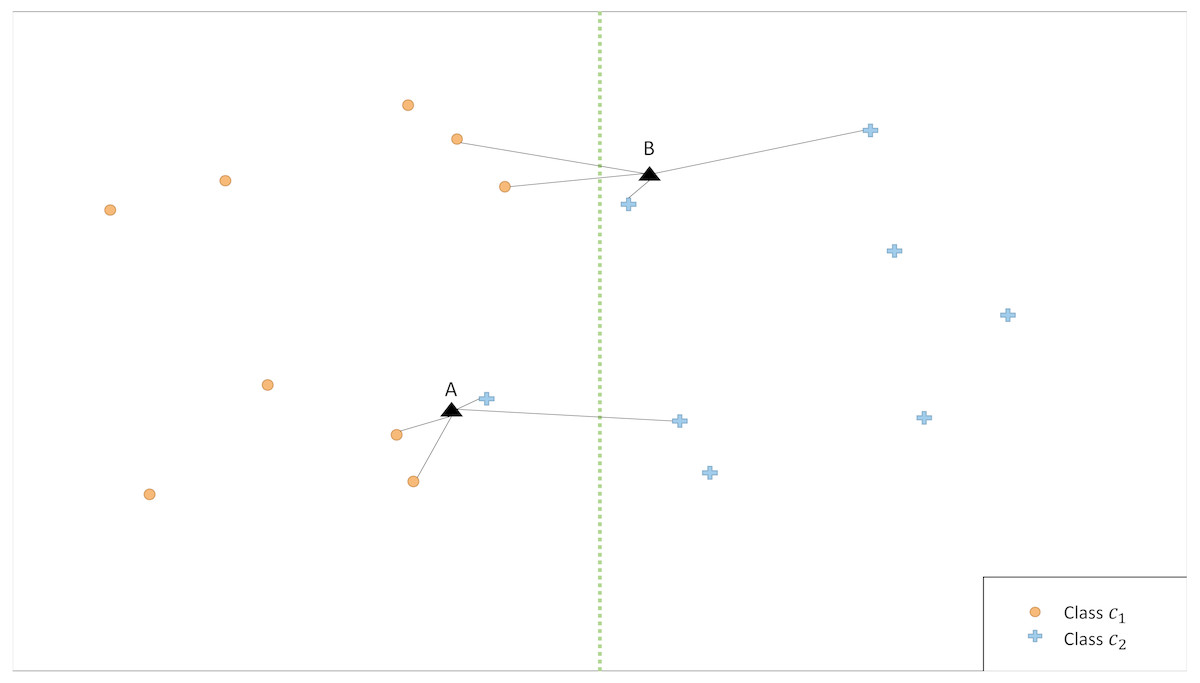
Figure 3: Illustration of classification by kCNN versus EkCNN.
The vertical line is the true class boundary and the target points A and B are to be classified. Based on the distance results, kCNN with k = 1(k = 2) only predicts B (A) correctly. On the other hand, EkCNN with k = 2 combines class probability for each k value and predicts both A and B correctly.
The complexity of EkCNN may be obtained analogously to steps (a)–(c) in ‘Time complexity of kCNN’. The complexities of EkCNN required in step (a) and (b) are the same as those of kCNN. In step (c), EkCNN requires O(kL) sum and comparison operations. Hence, the complexity of EkCNN is O(Nq + Nk + kL).
Experimental Evaluation
Data sets
We evaluated the proposed approaches using real benchmark data sets available at the UCI machine learning repository (Lichman, 2013). (We chose data sets to be diverse; all data sets we tried are shown.) Table 1 shows basic statistics of each data set including its numbers of classes and features. All data sets are available online at: https://archive.ics.uci.edu/ml/datasets.html. The data sets are ordered by the number of instances.
| Name | Features | Classes | Instances | Class distributions |
|---|---|---|---|---|
| Voice | 309 | 2 | 126 | 84/42 |
| Wine | 13 | 3 | 178 | 71/59/48 |
| Parkins | 22 | 2 | 195 | 147/48 |
| Cancer | 24 | 2 | 198 | 151/47 |
| Sonar | 60 | 2 | 208 | 111/97 |
| Seeds | 7 | 3 | 210 | 70/70/70 |
| Haberman | 3 | 2 | 306 | 225/81 |
| Ecoli | 7 | 8 | 336 | 143/77/52/35/20/5/2/2 |
| Libras | 90 | 15 | 360 | 24/24/.../24/24 |
| Musk | 166 | 2 | 476 | 269/207 |
| Blood | 4 | 2 | 748 | 570/178 |
| Diabetes | 8 | 2 | 768 | 500/268 |
| Vehicle | 18 | 4 | 846 | 218/217/212/199 |
| German | 24 | 2 | 1,000 | 700/300 |
| Yeast | 8 | 10 | 1,484 | 463/429/224/163/51/44/35/30/20/5 |
| Handwritten | 256 | 10 | 1,593 | 1,441/152 |
| Madelon | 500 | 2 | 2,000 | 1,000/1,000 |
| Image | 19 | 7 | 2,310 | 330/330/.../330/330 |
| Wave | 21 | 2 | 5,000 | 1,696/1,657/1,647 |
| Magic | 10 | 2 | 19,020 | 12,332/6,688 |
Experimental setup
We compared kCNN and EkCNN against kNN, WkNN, PNN, LMkNN and MLM-kHNN. Moreover, we considered an ensemble version of kNN (EkNN). EkNN estimates the probability for class ci as where is the probability estimated by kNN based on w nearest neighbors. Since MLM- kHNN is an ensemble of LMkNN using the harmonic mean, no additional ensemble model was considered. For EkCNN, we used r = q where q is the number of features of the data set. For kCNN and EkCNN, we added ϵ = 10−7 to each distance in equation Eq. (4) to avoid dividing by zero when the distance is zero.
For evaluation, we choose error rate (or equivalently accuracy), since error rate is one of the most commonly used metric and the skewness of the class distribution is not severe for most of the chosen data sets. The percentage of the majority class is less than 80% for most data sets (19 out of 20 data sets).
The analysis was conducted in R (R Core Team, 2014). For assessing the performance of the classifiers, we used 10-fold cross validation for each data. In the experiments, we varied the size of the neighborhood k from 1 to 15. For each method except PNN, the optimal value of k has to be determined based on the training data only. To that end, each training fold of the cross-validation (i.e., 90% of the data) was split into two random parts: internal training data (2/3) and internal validation data (1/3). The optimal k was the value that minimized classification error on the internal validation set. For PNN, Markov Chain Monte Carlo (MCMC) simulated samples are required. Following Holmes & Adams (2002), we used 5,000 burn-in samples, and retained every 100th sample in the next 50,000 samples.
We applied the Wilcoxon signed-rank test (Wilcoxon, 1945; Demšar, 2006) to carry out the pairwise comparisons of the methods over multiple data sets because unlike the t–test it does not make a distributional assumption. Also, the Wilcoxon test is more robust to outliers than the t-test (Demšar, 2006). The Wilcoxon test results report whether or not any two methods were ranked differently across data sets. Each test was one-sided at a significance level of 0.05.
Results
Table 2 summarizes the error rate (or misclassification rate) of each approach on each data set. Parameter k was tuned separately for each approach. EkCNN performed best on 8 out of the 20 data sets and kCNN performed best on 2 data sets. EkCNN achieved the lowest (i.e., best) average rank and kCNN the second lowest average rank. In the cases where kCNN performed the best, EkCNN was the second best method. According to the Wilcoxon test, EkCNN had a significantly lower (i.e., better) rank than kNN, EkNN, WkNN, LMkNN and kCNN with p-values less than 0.01. There was marginal evidence that EkCNN had a lower average rank than MLM- kHNN (p-value = 0.0656). Also, kCNN performed significantly better than kNN (p-value = 0.001), EkNN (p-value = 0.003), WkNN (p-value = 0.024), PNN (p-value = 0.003) and LMkNN (p-value = 0.041).
| kNN | EkNN | WkNN | PNN | LMkNN | MLM- kHNN | kCNN | EkCNN | |
|---|---|---|---|---|---|---|---|---|
| Voice | 0.3598 | 0.3625 | 0.3990 | 0.3701 | 0.4060 | 0.4316 | 0.3675 | 0.3941 |
| Wine | 0.2871 | 0.2748 | 0.2871 | 0.3110 | 0.2819 | 0.2361 | 0.2770 | 0.2534 |
| Parkins | 0.1783 | 0.1583 | 0.1750 | 0.1921 | 0.1983 | 0.1833 | 0.1783 | 0.1710 |
| Cancer | 0.2782 | 0.3130 | 0.2942 | 0.2675 | 0.3006 | 0.2927 | 0.2524 | 0.2410 |
| Sonar | 0.1815 | 0.1815 | 0.1815 | 0.2443 | 0.1820 | 0.1534 | 0.1767 | 0.1666 |
| Seeds | 0.1500 | 0.1500 | 0.1500 | 0.1423 | 0.0952 | 0.1000 | 0.1000 | 0.0901 |
| Haberman | 0.2769 | 0.2952 | 0.3128 | 0.2740 | 0.3305 | 0.3388 | 0.2572 | 0.2604 |
| Ecoli | 0.1365 | 0.1320 | 0.1370 | 0.1442 | 0.1482 | 0.1335 | 0.1394 | 0.1305 |
| Libras | 0.1528 | 0.1528 | 0.1428 | 0.1405 | 0.1500 | 0.1320 | 0.1360 | 0.1320 |
| Musk | 0.1493 | 0.1444 | 0.1182 | 0.1440 | 0.0832 | 0.0849 | 0.1388 | 0.1078 |
| Blood | 0.2438 | 0.2456 | 0.2397 | 0.2407 | 0.2433 | 0.3208 | 0.2432 | 0.2207 |
| Diabetes | 0.2643 | 0.2798 | 0.2736 | 0.2605 | 0.2629 | 0.2759 | 0.2616 | 0.2560 |
| Vehicle | 0.3666 | 0.3373 | 0.3721 | 0.3718 | 0.3028 | 0.3087 | 0.3643 | 0.3560 |
| German | 0.3200 | 0.3220 | 0.3312 | 0.3150 | 0.3200 | 0.3120 | 0.3020 | 0.3100 |
| Yeast | 0.4192 | 0.4291 | 0.4021 | 0.4024 | 0.4219 | 0.4200 | 0.4152 | 0.3943 |
| Handwritten | 0.0891 | 0.0752 | 0.0744 | 0.0901 | 0.0478 | 0.0415 | 0.0881 | 0.0625 |
| Madelon | 0.2733 | 0.2905 | 0.2939 | 0.2700 | 0.3209 | 0.3592 | 0.2625 | 0.2601 |
| Image | 0.0346 | 0.0366 | 0.0330 | 0.0524 | 0.0337 | 0.0316 | 0.0346 | 0.0346 |
| Wave | 0.1590 | 0.1664 | 0.1674 | 0.1320 | 0.1522 | 0.1606 | 0.1478 | 0.1520 |
| Magic | 0.1856 | 0.1833 | 0.1826 | 0.1890 | 0.1962 | 0.1859 | 0.1854 | 0.1780 |
| Average | 0.2253 | 0.2265 | 0.2284 | 0.2277 | 0.2239 | 0.2251 | 0.2164 | 0.2085 |
| Ranking | 5.25 | 5.38 | 5.08 | 5.05 | 5.22 | 4.35 | 3.55 | 2.13 |
Equation (4) contains a tuning parameter r. As mentioned above, increasing r smoothes posterior estimates. For the results of EkCNN presented in Table 2, we chose r = q for all data sets. While not shown here, using r = q resulted in lower or equal error rates compared with using r = 1 on 18 out of 20 data sets. Specifying r = q reduced the error rate up to 6% relative to the error rate for r = 1.
Illustrating the choice of r on the sonar data set
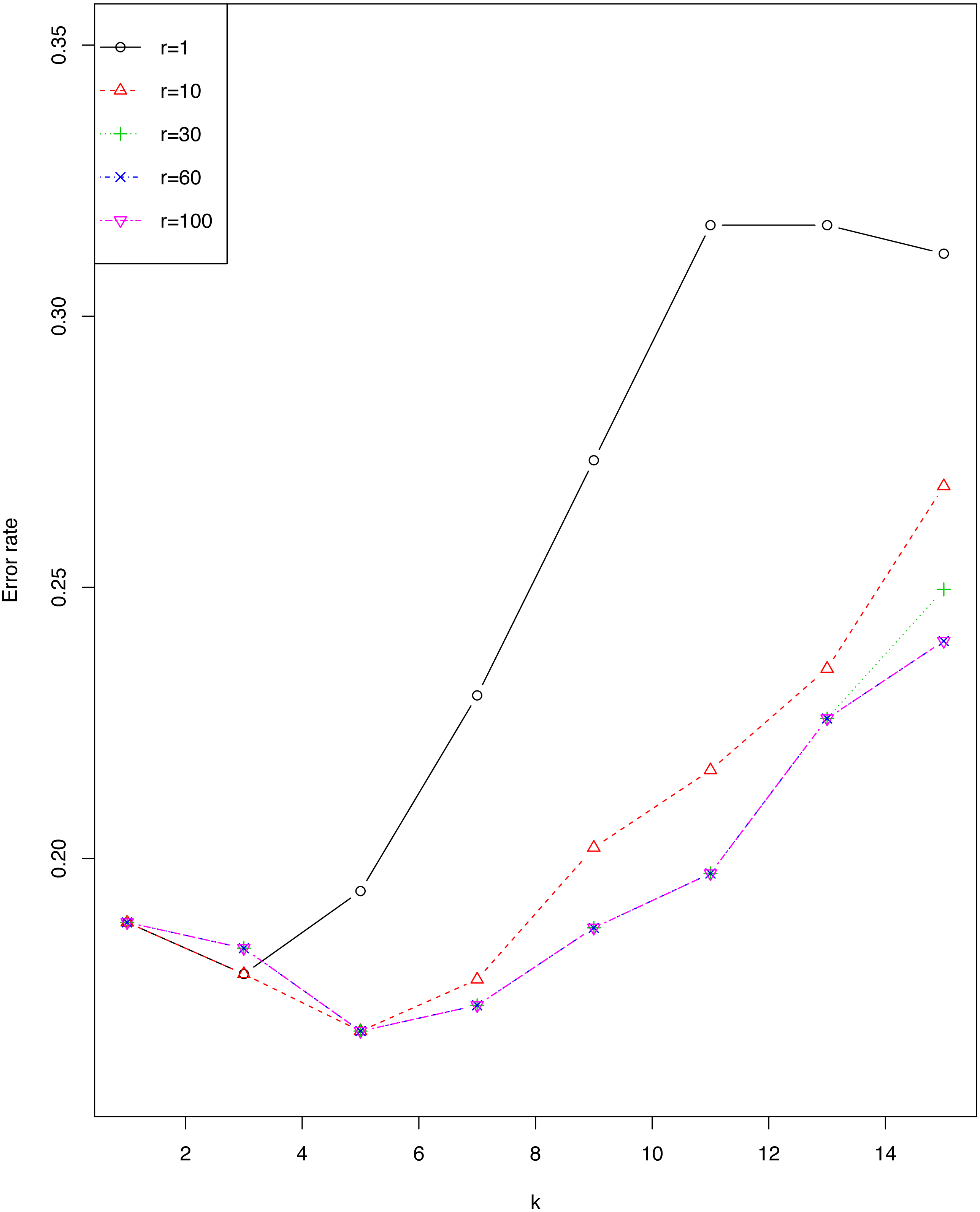
We investigated the impact of r and ϵ on error rate of EkCNN (Classification by kCNN is affected by neither r nor ϵ.) for the sonar data set. Figure 4 shows that the error rate varied little for small values of k. For this data set, larger values of r are consistently preferable to smaller values. Note that error rates for r = 60 were almost identical to those for r = 100.
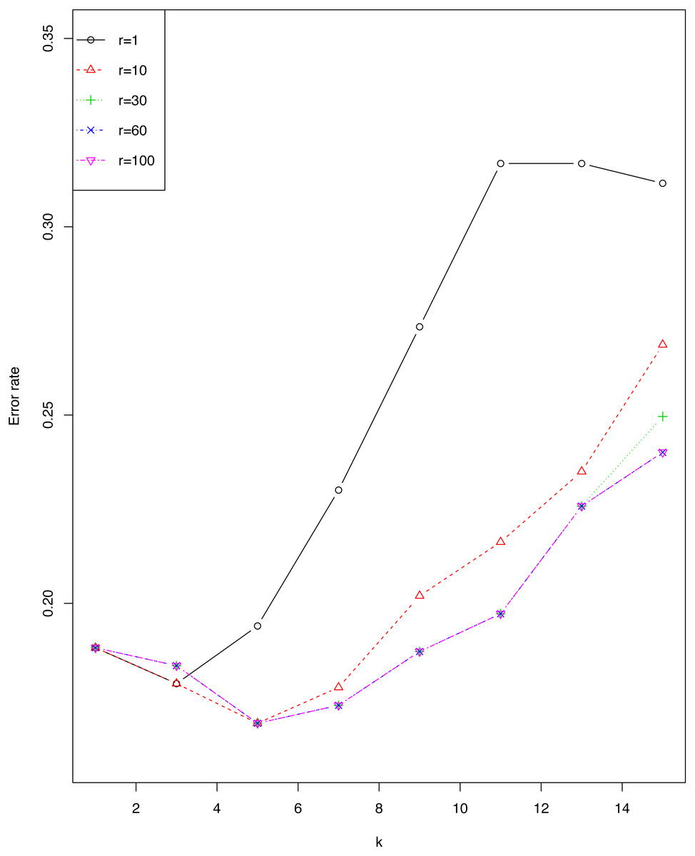
Figure 4: Impact of the tuning parameter r on error rates using the sonar data set.
Exploring Properties of the Proposed Method
In the following subsections, we investigate kCNN’s decision boundary and posterior probability using simulation. Further, we also discuss where kCNN beats kNN for posterior estimation.
Decision boundary of kCNN and EkCNN with varying k
This section illustrates that the decision boundary between classes is smoother as k increases for both kCNN and EkCNN. We used a simulated data set from Friedman, Hastie & Tibshirani (2001). The classification problem contains two classes and two real valued features.
Figure 5 shows the decision boundary of kCNN with different k (solid curve) and the optimal Bayes decision boundary (dashed red curve). Increasing k resulted in smoother decision boundaries. However, when k is too large (e.g., k = 30 in this example), the decision boundary was overly smooth.
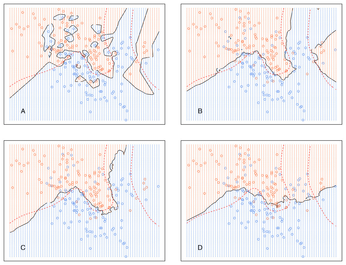
Figure 5: kCNN on the simulated data with different choices of k.
The broken red curve is the Bayes decision boundary. (A) kCNN (k = 1), (B) kCNN (k = 5), (C) kCNN (k = 10), (D) kCNN (k = 30).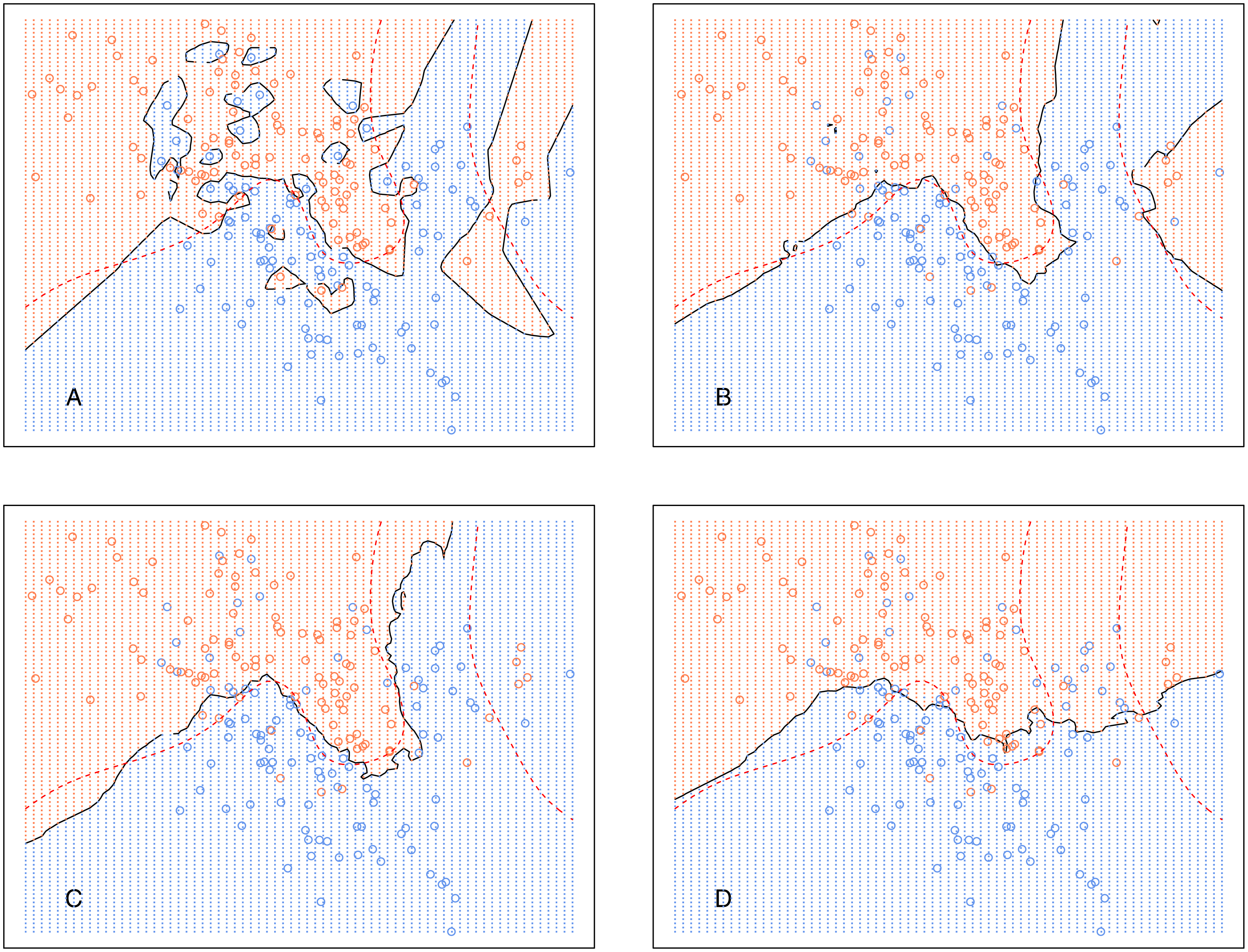
Analogously, Fig. 6 shows the decision boundary of EkCNN at r = 2 and different values k. Similar to kCNN, the decision boundary was smoothed as k increased. However, the magnitude of the changes was less variable. For example, the decision boundaries of EkCNN at k = 10 and k = 30 were similar, while those of kCNN were quite different.
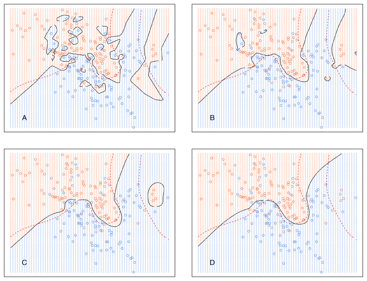
Figure 6: EkCNN on the simulated data with different choices of k.
The broken red curve is the Bayes decision boundary. (A) EkCNN (k = 1), (B) EkCNN (k = 5), (C) EkCNN (k = 10), (D) EkCNN (k = 30).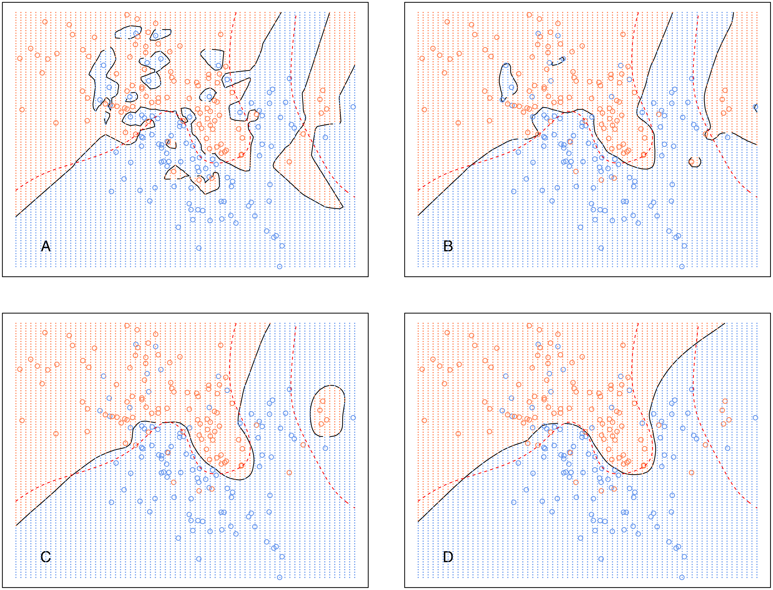
Comparison of the posterior probability distribution of kNN and kCNN
Rather than considering classification, this section compares kCNN with kNN in terms of posterior probabilities. Probabilities are of interest, for example, when evaluating the entropy criterion. Using the same data set as in ‘Decision boundary of kCNN and EkCNN with varying k’, we plot the full posterior probability contours of kNN and kCNN in Fig. 7. We set r = q = 2 for kCNN. For k = 1, as expected, the posteriors estimated by kNN was always either 0 or 1. By contrast, kCNN provided less extreme posterior results even at k = 1. The posterior probabilities changed more gradually.
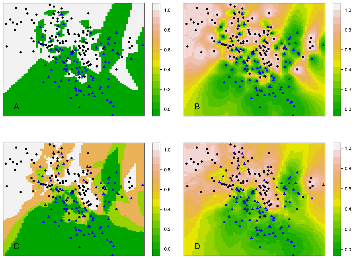
Figure 7: Contour plots of posterior probabilities of kNN and kCNN for k = 1 and k = 3.
(A) kNN (k = 1), (B) kCNN (k = 1), (C) kNN (k = 3), (D) kCNN (k = 3).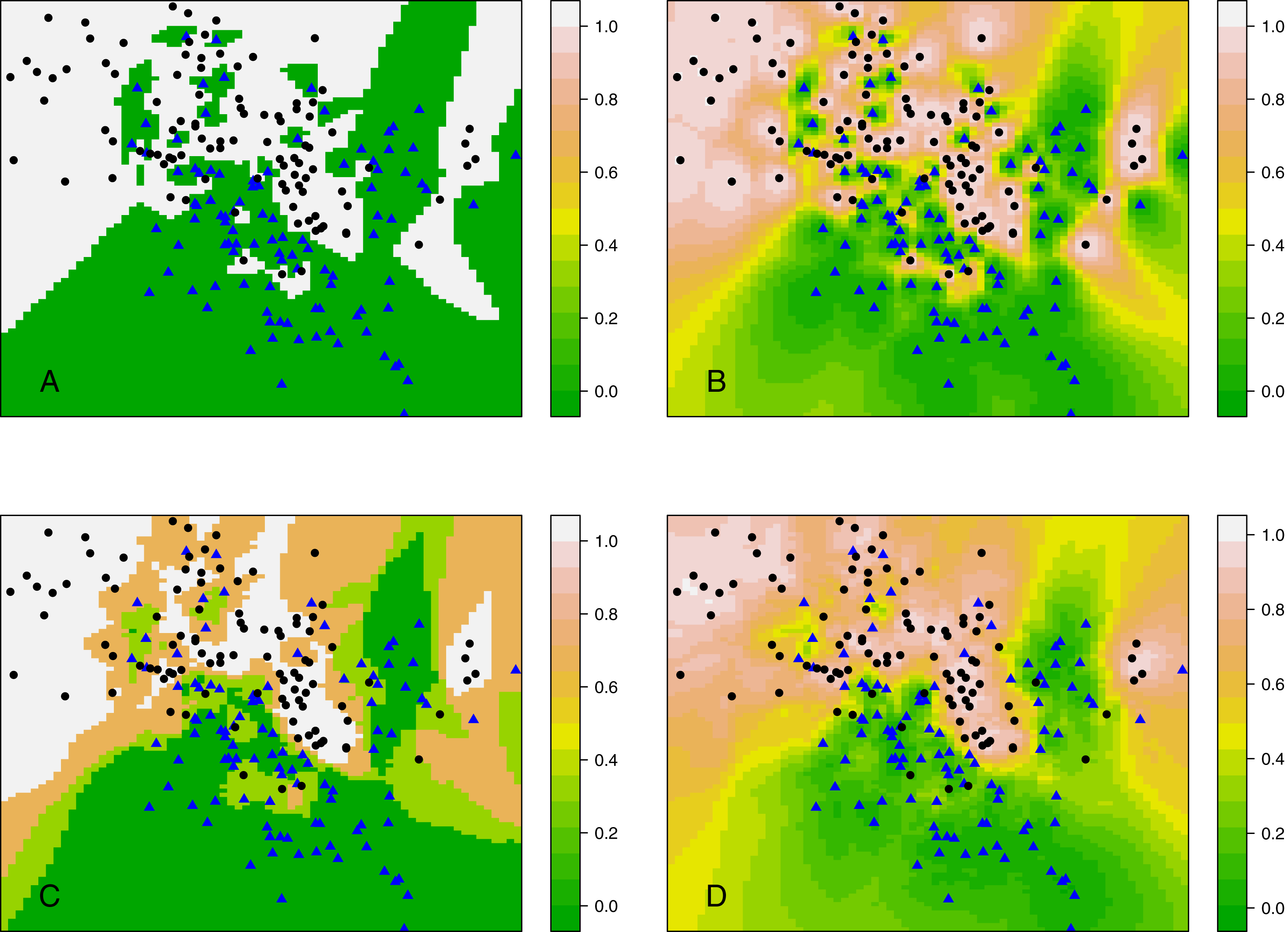
When k = 3, posterior probabilities from kNN jumped between four possible values (0, 1/3, 2/3, 1), whereas those from kCNN were much smoother. The result shows that unlike kNN, kCNN can produce smooth posterior probability fields even at small values of k.
Under what circumstances does the proposed method beat kNN?
kCNN (or EkCNN) may be useful when the true posterior distribution has a full range of probabilities rather than near dichotomous probabilities (close to 0 or 1). This occurs when the distributions of the classes substantially overlap. When the distribution of each class is well separated, for any data point the classification probabilities will be (near) 1 for one class and (near) 0 for the other classes. Otherwise, when the distributions overlap, the classification probabilities will be less extreme.
We conducted a small simulation to illustrate that kCNN is preferable to kNN when k is small and the distributions of the classes overlap. Assume that instances from each class are independently distributed following a multivariate normal distribution. Denote by μi the mean vector and by ∑i the covariance matrix of class ci. The parameters were given as where Iq is the q dimensional identity matrix. Note that s is the Euclidean distance between the two means. Therefore, s controls the degree of overlap between the distributions of the two classes.
In order to obtain less variable results, we used 10 independent replicates for each parameter setting. The final outputs were obtained by averaging the results. We used 100 training and 1,000 test instances and the equal prior setting for the classes. Like Wu, Lin & Weng (2004), we evaluated the posterior estimates based on mean squared error (MSE). The MSE for the test data is obtained as where xj represents the jth test instance.
Table 3 shows the MSE for each method as a function of s and k when p = 2. The kCNN method beat kNN for small values of s. Small values of s imply that the mean vectors are close to each other, and hence there is more overlap between the two conditional densities. The difference in performance between the two methods decreased as s or k increased.
| k = 1 | k = 5 | k = 10 | k = 20 | |||||
|---|---|---|---|---|---|---|---|---|
| s | kNN | kCNN | kNN | kCNN | kNN | kCNN | kNN | kCNN |
| 0.1 | 0.504 | 0.074 | 0.115 | 0.017 | 0.065 | 0.011 | 0.038 | 0.006 |
| 0.5 | 0.483 | 0.080 | 0.094 | 0.022 | 0.046 | 0.019 | 0.025 | 0.016 |
| 1 | 0.449 | 0.113 | 0.082 | 0.054 | 0.042 | 0.053 | 0.028 | 0.058 |
| 1.5 | 0.308 | 0.104 | 0.056 | 0.064 | 0.024 | 0.073 | 0.016 | 0.085 |
| 2 | 0.211 | 0.096 | 0.045 | 0.082 | 0.024 | 0.094 | 0.016 | 0.113 |
Next, we considered the effect of feature dimension q on each method. Table 4 shows the MSE for each method as a function of q and k when s = 0.1. Throughout the range of q, kCNN outperformed kNN. As q increased the MSE for kCNN was less affected by the choice of k.
| k = 1 | k = 5 | k = 10 | k = 20 | |||||
|---|---|---|---|---|---|---|---|---|
| q | kNN | kCNN | kNN | kCNN | kNN | kCNN | kNN | kCNN |
| 2 | 0.502 | 0.070 | 0.122 | 0.014 | 0.054 | 0.006 | 0.022 | 0.004 |
| 5 | 0.499 | 0.017 | 0.100 | 0.003 | 0.048 | 0.002 | 0.021 | 0.002 |
| 10 | 0.503 | 0.007 | 0.112 | 0.003 | 0.058 | 0.002 | 0.027 | 0.002 |
| 30 | 0.500 | 0.002 | 0.102 | 0.002 | 0.053 | 0.001 | 0.026 | 0.001 |
| 50 | 0.494 | 0.002 | 0.103 | 0.001 | 0.049 | 0.001 | 0.023 | 0.001 |
Application: Semi-automated Classification Using the Patient Joe Text Data
In the previous section, we discussed situations where the proposed method is preferred over kNN. This section shows that the proposed algorithm is useful in the semi-automatic classification of text data. In semi-automatic text classification, high prediction accuracy is more important than fully automating classification; since somewhat uncertain predictions are manually classified. We first distinguish between easy-to-categorize and hard-to-categorize text instances. The easy-to-categorize texts are classified by statistical learning approaches, while the hard-to-categorize instances are classified manually. This is needed especially for text data from open-ended questions in the social sciences, since it is difficult to achieve high overall accuracy with full automation and manual classification is time-consuming and expensive.
The goal in semi-automatic classification is to obtain high classification accuracy for a large number of text instances. Hence, a classifier needs to not only predict the correct classes but also well order the text instances by the difficulty of classification.
For our application, we used a survey text data set (Martin et al., 2011) (we call the data set “Patient Joe”). The data were collected as follows. The respondents were asked to answer the following open-ended question: “Joe’s doctor told him that he would need to return in two weeks to find out whether or not his condition had improved. But when Joe asked the receptionist for an appointment, he was told that it would be over a month before the next available appointment. What should Joe do?” In 2012, the Internet panel LISS (http://www.lissdata.nl) asked the question in Dutch and classified the text answers into four different classes (proactive, somewhat proactive, passive and counterproductive). See Martin et al. (2011) and Schonlau & Couper (2016) for more information about the data set.
The original texts were converted to sets of numerical variables (preprocessing). Briefly, we created an indicator variable for each word (unigram). The variable indicates whether or not the word is present in a text answer. Then a text answer was represented by a binary vector (each dimension represents a word). After converting the text answers in the Patient Joe data set, we had 1758 instances with 1,750 total unigrams.
In semi-automated classification, test instances are ordered from the easiest-to-categorize instance to the hardest-to-categorize instance based on the probability estimate of the predicted class.
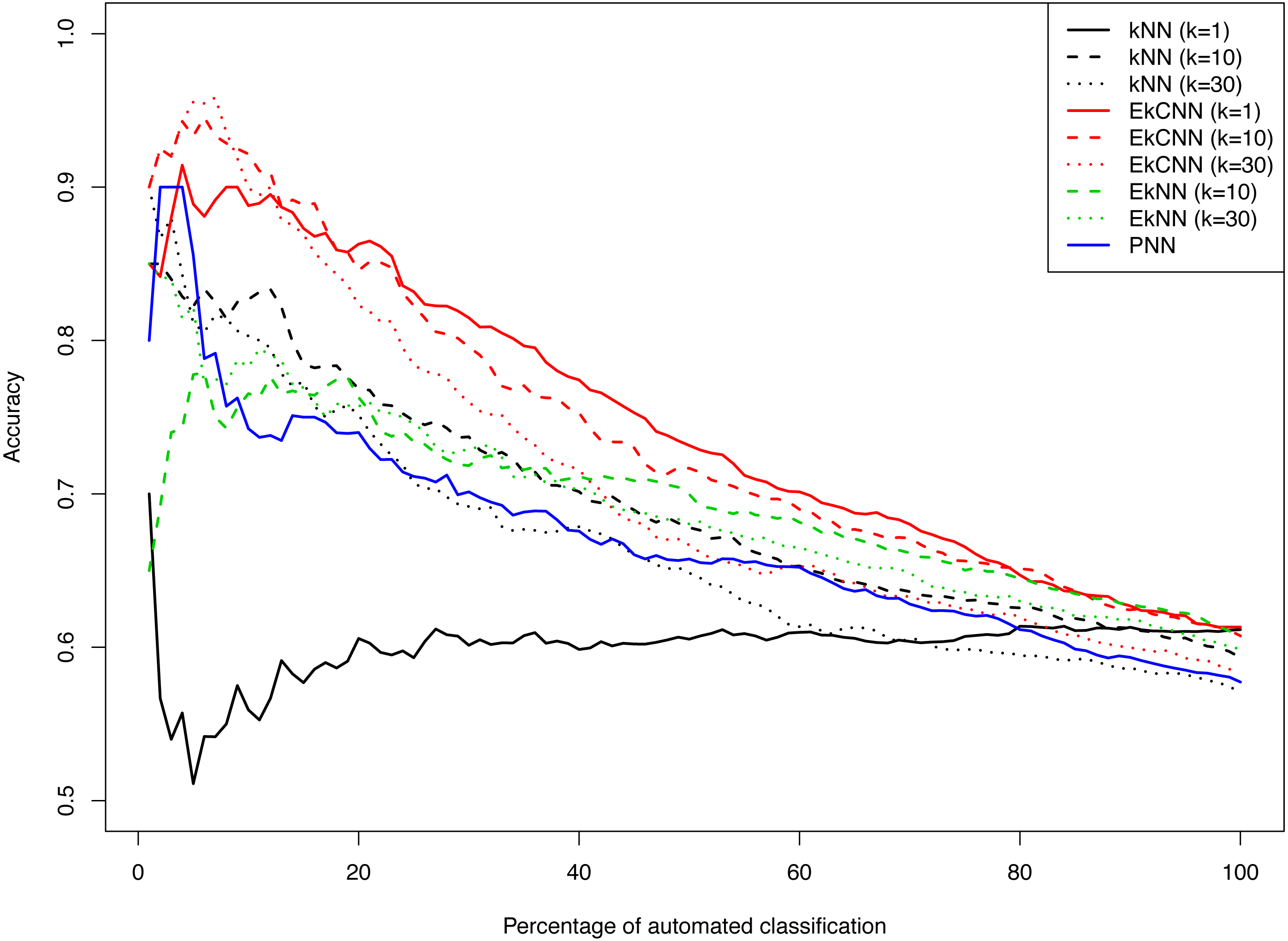
Figure 8 shows the accuracy of kNN, EkNN and EkCNN (at k = 1, 10 and 30) and PNN as a function of the percentage of the test data that were classified automatically by each method. (The other nearest neighbor based approaches, LMkNN and MLM-kHNN, do not produce class probabilities, and thus were excluded in the comparison.) Also, since EkNN and kNN is equivalent at k = 1, the column for EkNN with k = 1 is omitted. In most cases, high accuracy was achieved when only a small percentage of text answers were classified. However, as the percentage of automated classification increased and more hard-to-categorize instances are included, accuracy tended to decrease. There was one exception: for kNN with k = 1, accuracy did not increase as the probability threshold for automatic classification increased. That is because for kNN at k = 1 probability 1 is assigned to the class of the nearest neighbor for each test instance. In other words, for k = 1 kNN failed to prioritize the text answers. The EkCNN method, however, ordered the test instances well even at k = 1.EkCNN with k = 1 resulted in higher accuracy than k = 10 or k = 30 when more than 20% of the data were classified automatically. From the figure it is clear that EkCNN achieved higher accuracy than kNN at almost all percentages regardless of the values of k. Equivalently, at a target accuracy, a larger number of the text answers could be classified by EkCNN. Also EkCNN at any value of k outperformed PNN. The differences in accuracy between the methods tended to be larger at lower percentages of automated classification, i.e., when a substantial percentage of text was manually classified, which is typical in semi-automated classification of open-ended questions. In semi-automated classification this would lead to cost savings. The results are summarized in Table 5. EkCNN was preferred to kNN, EkNN and PNN for semi-automated classification of the Patient Joe data.
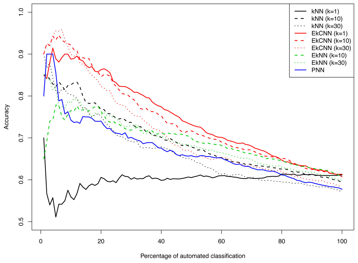
Figure 8: Comparison of kNN, EkNN, PNN and EkCNN with different choices of k for semi-automatic classification on the Patient Joe data.
| Percentage of Automated Classification | Accuracy | ||||||||
|---|---|---|---|---|---|---|---|---|---|
| kNN | EkNN | EkCNN | PNN | ||||||
| k = 1 | k = 10 | k = 30 | k = 10 | k = 30 | k = 1 | k = 10 | k = 30 | ||
| 10% | 0.5591 | 0.8267 | 0.80291 | 0.7653 | 0.7826 | 0.8909 | 0.9215 | 0.8993 | 0.7424 |
| 20% | 0.6057 | 0.7685 | 0.7514 | 0.7628 | 0.7571 | 0.8628 | 0.8457 | 0.8228 | 0.7400 |
| 30% | 0.6013 | 0.7371 | 0.69172 | 0.7184 | 0.7296 | 0.8147 | 0.7957 | 0.7598 | 0.7013 |
| 40% | 0.6005 | 0.7014 | 0.6785 | 0.7114 | 0.7042 | 0.7742 | 0.7528 | 0.7157 | 0.6757 |
| 50% | 0.6052 | 0.6779 | 0.6484 | 0.6996 | 0.6803 | 0.7315 | 0.7166 | 0.6666 | 0.6575 |
| 100% | 0.6115 | 0.5932 | 0.5710 | 0.6086 | 0.5990 | 0.6132 | 0.6074 | 0.5841 | 0.5934 |
Discussion
For the 20 benchmark data sets, EkCNN had the lowest and kCNN the second lowest average error rate. In terms of statistical significance, EkCNN performed significantly better than kNN, EkNN, WkNN, PNN, LMkNN and kCNN on error rate. For the same data sets, kCNN performed significantly better than kNN, EkNN, WkNN, PNN and LMkNN.
The ensemble method EkCNN performed better than kCNN. For each k, kCNN uses a single posterior estimate for each class, whereas EkCNN combines multiple posterior estimates. This more differentiated estimate for posteriors may be the reason for the greater classification accuracy. We therefore recommend EkCNN over kCNN for higher classification accuracy.
We have shown that kCNN is asymptotically Bayes optimal for r = 1. It is interesting that for the ensemble version EkCNN, r = q is clearly preferable. While surprising, there is no contradiction: the Bayes optimality only applies asymptotically and only for kCNN and not for the ensemble version EkCNN.
While the tuning parameter r does not affect classification for kCNN, r does affect classification for EkCNN. For the empirical results presented in Table 2, we chose r = q for all data sets. We also noted that in 18 of the 20 data sets r = q leads to a lower or equal error rate as compared to r = 1. Rather than just tuning the parameter k, it would be possible to simultaneously tune k and r. While this may further improve the error rates of EkCNN, the improvement, if any, would come at additional computational cost and is not expected to be appreciably large. For example, for the sonar data set, we have demonstrated in ‘Illustrating the choice of r on the sonar data set’ that no improvement was obtained when r > q.
The simulation study in ‘Decision boundary of kCNN and EkCNN with varying k’ showed that the decision boundary obtained by kCNN can be smoothed by increasing k. Although this result seems similar to that of kNN, the reasons for smoothed decision boundaries are different. As k increases, kNN considers more observations for classification and thus the classification is less affected by noise or outliers. By contrast, kCNN always uses the same number of observations (the number of classes) to make a prediction regardless of k. The kCNN approach ignores the first k − 1 nearest neighbors from each class and this makes the decision boundary less local.
Since EkCNN is a combination of multiple kCNN classifiers, its decision boundary is also a combined result of multiple decision boundaries from kCNN. Because the decision boundary obtained by kCNN is smoothed as k increases, that obtained by EkCNN is also smoothed. However, the smoothing occurs more gradually, since the decision boundary obtained at k is always combined with the k − 1 less smooth decision boundaries. This implies that EkCNN is more robust than kCNN against possible underfitting that may occur at large k. The decision boundaries shown in ‘Decision boundary of kCNN and EkCNN with varying k’ confirmed this.
An advantage of the proposed methods over kNN, especially when k is low, is that kCNN (or EkCNN) can estimate more fine-grained probability scores than kNN, even at low values of k. For kNN, a class probability for a new observation is estimated as the fraction of observations classified as that class. By contrast, kCNN estimates the posteriors based on distances. We confirmed this in ‘Comparison of the posterior probability distribution of kNN and kCNN’ using simulated probability contour plots.
A simulation in ‘Under what circumstances does the proposed method beat kNN?’ suggests that the greater the overlap among the posterior distribution of each class, the more likely that kCNN beats kNN in terms of the MSE. In most applications class distributions overlap, which partially explains why in the experiment in ‘Result’ kCNN performed better than kNN in many cases.
The application in ‘Application: Semi-automated Classification Using the Patient Joe Text Data’ showed that EkCNN outperformed kNN and PNN in semi-automated classification, where easy-to-categorize and hard-to-categorize instances need to be separated. When only a percentage of the text data was classified automatically (as is typical in semi-automatic classification), EkCNN achieved higher accuracy than the other two approaches.
Like all nearest neighbor approaches, limitations of kCNN include lack of scalability to very large data sets.
Conclusion
In this paper, we have proposed a new nonparametric classification method, kCNN, using conditional nearest neighbors. We have demonstrated that kCNN is an approximation of the Bayes classifier. Moreover, we have shown that kCNN converges in probability to the Bayes optimal classifier as the number of training instances increase. We also considered an ensemble of kCNN called EkCNN. The proposed methods compared favorably to other nearest neighbor based methods on some benchmark data sets. While not beating all competitors on all data sets, the proposed classifiers are promising algorithms when facing a new prediction task. Also, the proposed methods are especially advantageous when class probability estimations are needed and when the class distributions highly overlap. The proposed method appears especially useful for semi-automated classification.