
Vertical distribution of megafauna on the Bering Sea slope based on ROV survey
- Published
- Accepted
- Received
- Academic Editor
- Blanca Figuerola
- Subject Areas
- Biodiversity, Biogeography, Ecology, Marine Biology, Zoology
- Keywords
- Bering Sea, ROV survey, Vertical distribution, Vertical zonation, Megafauna, Volcanologists Massif, Komandorsky Basin, Biodiversity
- Copyright
- © 2020 Rybakova et al.
- Licence
- This is an open access article distributed under the terms of the Creative Commons Attribution License, which permits unrestricted use, distribution, reproduction and adaptation in any medium and for any purpose provided that it is properly attributed. For attribution, the original author(s), title, publication source (PeerJ) and either DOI or URL of the article must be cited.
- Cite this article
- 2020. Vertical distribution of megafauna on the Bering Sea slope based on ROV survey. PeerJ 8:e8628 https://doi.org/10.7717/peerj.8628
Abstract
Video surveys were carried out during the 75th cruise of the RV Akademik M.A. Lavrentyev (June 2016) along the northern slope of the Volcanologists Massif, in the south-western Bering Sea. The seafloor was explored using the ROV Comanche 18. Seven dives were performed in the depth range from 4,278 m to 349 m. Overall, about 180 species of megafauna were recognised. Fifteen types of megafauna communities corresponding to certain depth ranges were distinguished based on the most abundant taxa. Dominance changed with depth in the following order: the holothurian Kolga kamchatica at the maximum depth (4,277–4,278 m); the holothurian Scotoplanes kurilensis at 3,610–2,790 m; the ophiuroid Ophiura bathybia at 3,030–2,910 m; benthic shrimps of the family Crangonidae at 2,910–2,290 m; the holothurian Paelopatides solea at 2,650–2,290 m; benthic jellyfish from the family Rhopalonematidae at 2,470–2,130 m; the enteropneust Torquaratoridae at 2,290–1,830 m; the holothurian Synallactes chuni and the ophiuroid of the genera Ophiura and Ophiocantha at 1,830–1,750 m. At depths 1,750–720 m most of the megafauna was associated with live or dead colonies of the sponge Farrea spp. Depths 720–390 m were dominated by the coral Heteropolypus ritteri and/or Corallimorphus pilatus. At 390–350 m depth, the shallowest depth range, the dominant taxon was the zoantharian Epizoanthus sp. Soft sediment megafauna communities dominated by torquaratorid enteropneusts to our knowledge have not been observed before in the deep-sea, the same as communities with a dominance of benthopelagic rhopalonematid jellyfish. The depths of the largest community changes, or the largest turnover of dominant species, were revealed at ∼2,790 m between the bathyal and abyssal zones and ∼1,750 m and ∼720 m within the bathyal zone.
Introduction
Depth plays a crucial role in the distribution of species and communities in the World Ocean. It was shown that species generally occupy discrete depth ranges and progressively replace each other from the continental shelf to the abyssal depths (Carney, Haedrich & Rowe, 1983). Distinct bathymetric faunal zones have been identified for many marine taxa (Mironov, 1986; Billett, 1991; Cartes & Sarda, 1993) and for marine fauna in general (Rowe & Menzies, 1969; Menzies, George & Rowe, 1973; Haedrich, Rowe & Polloni, 1975). Very few studies have examined the depth-related distribution of deep-sea species within their depth ranges to understand not only critical depths of faunal change but to identify more subtle changes that are related to the abundance of species that can provide a better overall picture of faunal zonation. For example, Howell, Billett & Tyler (2002) showed that asteroid species have very narrow centres of distribution in which they are abundant, despite much wider total adult depth ranges. Depth-related faunistic boundaries occur at many locations worldwide indicating that important controlling factors are present at these depths and that they may occur globally. Causes of the vertical zonation are related to the biology and physiology of the marine organisms and controlled by change with depth of some pivotal environmental parameters such as pressure, light, temperature and food availability (Menzies, George & Rowe, 1973; Rex, 1976; Carney, 2005; Rex & Etter, 2010). Generally, the causes of change in species composition with depth are complex, and several factors might interact, leading to the certain patterns observed in the each specific area (Soltwedel et al., 2009).
Benthic megafauna may be defined as marine animals exceeding 0.5–1 cm in size and recognizable on seafloor images (Grassle et al., 1975; Rex, 1981). Information on abundance and distribution of the megafauna is important for deep-sea benthic ecology. Megafaunal organisms play an important role in benthic ecosystems through active recycling of sediment organic matter, bioturbation and food web linkages.
The number of megafaunal studies has increased with the growing use of deep-sea video and imagery for ecological purposes.
Investigation of the Bering Sea began in the 18th century by G.W. Steller during the V. Bering expedition (1,737–1,742). Various species from the Bering Sea were studied in the late 19th and early 20th century. The first quantitative results of the benthos distribution were obtained in 1,932–1,933 by K. Derugin (Ushakov & Kusakin, 1978). Further considerable contributions were made by expeditions of the RV Vityaz in 1,950–1,952 to the western part of the Bering Sea and by the expeditions of a number of research vessels in 1,958–1,960 to the eastern part of the Bering Sea (Ushakov, 1952; Vinogradova, 1954; Neyman, 1960; Neiman, 1963; Zenkevitch, 1963; Filatova & Barsanova, 1964; Kuznetzov, 1964; Semenov, 1964; Vinogradov & Neyman, 1965). Qualitative and quantitative studies of the distribution of the benthos and trophic structure were described mainly on the shelf and upper slope (Rowland, 1973; Stoker, 1973; Alton, 1974; Haflinger, 1978; Stoker, 1978; Jewett & Feder, 1981) while surveys of the Western (Komandorsky) and Central (Aleutian) Basins were extremely limited. Impact of climate change on the Bering Sea ecosystems is being actively studied; however, these investigations are restricted only to some economically important species and do not take into account benthic communities as a whole (Hamazaki et al., 2005; Grebmeier et al., 2006; Stevenson & Lauth, 2012). Available data on the deep basins of the Bering Sea were obtained using trawls and grabs. Image and video surveys of the deep-sea megafauna communities were not conducted before, with the exception of dives in the submersible Mir in 1990 to the Piip’s Volcano. Based on these dives, vertical zonation of benthic fauna on the upper part of the northern and southern slope of the Volcanologists Massif was described (Galkin & Sagalevich, 2012). It was mentioned about 30 species of megafauna in the depth range from 450 to 900 m and the vertical zonation in fauna distribution was revealed. Dominant taxa changed with depth with hexactinellid sponges in the lower part replaced by corals and unidentified small cnidarians in the upper part.
The Bering Sea is separated from the North Pacific Ocean by the Aleutian-Komandor Island systems. The channels between the islands often have a great depth, sometimes exceeding 4,000 m, permitting almost unrestricted exchange between the abyssal zone of the Bering Sea and the Pacific Ocean (Stoker, 1978). As a result, most of the deep-sea species of the Bering Sea are in common with the Pacific Ocean (Filatova & Barsanova, 1964). By contrast, the exchange with the Chukchi Sea and the Arctic Ocean is limited to the Bering Strait, less than 50 m deep. The biomass of benthos in the Komandorsky Basin is very high—up to 32 g/m2, average 14 g/m2 (Belyev, 1960). It is explained by favourable nutritional conditions due to proximity to the slope, abundant flora and fauna of the sublittoral zone and currents carrying organic-rich water from bays and mixing with the deep layers. For comparison, in the Central Basin biomass is lower due to isolation from the shelf (average 6 g/m2) (Filatova & Barsanova, 1964).
At least seven physical factors may influence the qualitative and quantitative distribution of the Bering Sea benthic fauna. These factors include sediment particle size, bottom temperature, salinity, depth, sedimentation rates, circulation intensity, and suspended particle content in the near-bottom water layer (Kuznetzov, 1964; Stoker, 1978). Usually species dominating faunal assemblages belong to several trophic groups (Neyman, 1960; Filatova & Barsanova, 1964; Stoker, 1973); however, one certain trophic type can prevail. The distribution of different trophic types depends on topography, distribution of organic carbon in the sediment, mobility of bottom waters and distribution of erosion and sedimented zones at the seafloor (Neiman, 1963; Rex, 1981; Gage & Tyler, 1991; Sokolova, 2000). For example, sessile suspension feeders are dominated in the Bering Sea at areas with high speed of currents, at areas with high concentrations of suspension particles in near bottom layers of water and on hard substrate (Kuznetzov, 1964). Deposit-feeders are dominated at areas with soft sediment enriched with organic carbon (Gage & Tyler, 1991).
The present study is the first detailed investigation on the megafauna communities of the slope of the Volcanologists Massif and adjacent area of the Komandorsky Basin based on video survey. Our main aim is to clarify patterns of the vertical distribution of megafauna communities on the slope of the Volcanologists Massif based on their composition and structure.
Material & Methods
Study area and video surveys
Video surveys were carried out during the 75th cruise of the RV Akademik M.A. Lavrentyev (June 2016) in the northern slope of the Volcanologists Massif, the south-west Bering Sea (Fig. 1). The seafloor was explored using the ROV Comanche 18 (Galkin & Ivin, 2019). Seven dives were performed in the depth range from 4,278 m to 349 m. For technical reasons, dives tracks were directed upwards along the slope. No specific permissions were required for the investigated location because it is the territorial waters of the Russian Federation and it is not the protected area.
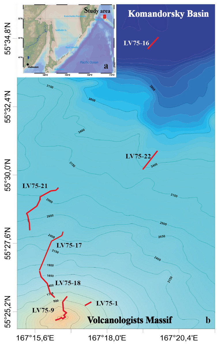
Figure 1: The tracks of the 7 ROV Comanche 18 dives on the northern slope of the Volcanologists Massif, in the south-west Bering Sea (75th cruise of RV Akademik M.A. Lavrentyev, June 2016).
Five of the dives are broken up further into quantitative transects as explained in Table 1.
Visual observations were conducted in a continuous mode, total duration is 40 hrs 44 min. Observations were accompanied by video recording and sampling of individual organisms by ROV manipulator. The field studies did not involve endangered or protected species. The ROV was equipped with the Kongsberg Underwater HDTV colour camera OE14-502 and with a ten-centimetre laser scale. A sonardyne USBL Fusion underwater navigation system was used. In total 22 hrs 29 min of video footage were analysed. Dive details are given in Table 1.
| Dive (#) | Date | Time on the bottom | Coordinates (observation) | Depth | Quantitative transect (#) | Duration (min:sec) | Estimated length (m) | Mean depth (m) | ||||||
|---|---|---|---|---|---|---|---|---|---|---|---|---|---|---|
| Start | End | Total (hour:min) | Start | End | Start | End | ||||||||
| Latitude (N) | Longitude (E) | Latitude (N) | Longitude (E) | |||||||||||
| 16 | 26.06.2016 | 17:57 | 21:08 | 3:11 | 55.5774 | 167.3258 | 55.5760 | 167.3249 | 4,278 | 4,277 | 1 | 3:07 | 144 | 4,277 |
| 2 | 3:40 | 169 | 4,277 | |||||||||||
| 3 | 2:24 | 111 | 4,277 | |||||||||||
| 4 | 1:36 | 74 | 4,277 | |||||||||||
| 22 | 02.07.2016 | 10:17 | 14:20 | 4:03 | 55.5143 | 167.3272 | 55.5039 | 167.3195 | 3,610 | 3,451 | 5 | 3:02 | 140 | 3,603 |
| 6 | 4:10 | 192 | 3,587 | |||||||||||
| 7 | 4:13 | 195 | 3,583 | |||||||||||
| 8 | 8:15 | 381 | 3,494 | |||||||||||
| 21 | 01.07.2016 | 10:34 | 19:32 | 8:58 | 55.4934 | 167.2726 | 55.4683 | 167.2537 | 3,023 | 2,502 | 9 | 8:00 | 370 | 2,983 |
| 10 | 5:00 | 232 | 3,023 | |||||||||||
| 11 | 5:00 | 232 | 2,954 | |||||||||||
| 12 | 5:00 | 232 | 2,960 | |||||||||||
| 13 | 5:00 | 232 | 2,890 | |||||||||||
| 14 | 5:00 | 232 | 2,890 | |||||||||||
| 15 | 5:05 | 235 | 2,849 | |||||||||||
| 16 | 3:40 | 169 | 2,847 | |||||||||||
| 17 | 4:40 | 216 | 2,847 | |||||||||||
| 18 | 5:00 | 232 | 2,790 | |||||||||||
| 19 | 5:00 | 232 | 2,732 | |||||||||||
| 20 | 5:00 | 232 | 2,626 | |||||||||||
| 21 | 5:00 | 232 | 2,555 | |||||||||||
| 22 | 3:00 | 139 | 2,502 | |||||||||||
| 23 | 5:00 | 232 | 2,502 | |||||||||||
| 17 | 27.06.2016 | 14:40 | 22:51 | 8:11 | 55.4665 | 167.2756 | 55.4438 | 167.2629 | 2,487 | 1,800 | 24 | 5:00 | 232 | 2,461 |
| 25 | 5:00 | 232 | 2,441 | |||||||||||
| 26 | 5:00 | 232 | 2,380 | |||||||||||
| 27 | 2:40 | 123 | 2,218 | |||||||||||
| 28 | 4:00 | 185 | 1,914 | |||||||||||
| 29 | 3:25 | 158 | 1,850 | |||||||||||
| 18 | 28.06.2016 | 9:45 | 15:59 | 6:14 | 55.4438 | 167.2628 | 55.4285 | 167.2699 | 1,806 | 992 | 30 | 6:00 | 277 | 1,785 |
| 31 | 2:40 | 123 | 1,750 | |||||||||||
| 32 | 2:30 | 115 | 1,650 | |||||||||||
| 33 | 2:30 | 115 | 1,600 | |||||||||||
| 1 | 11.09.2016 | 10:28 | 12:13 | 1:45 | 55.4242 | 167.2922 | 55.4251 | 167.2905 | 1,077 | 1,055 | – | – | – | |
| 9 | 19.06.2016 | 10:38 | 19:00 | 8:22 | 55.4289 | 167.2779 | 55.4299 | 167.2773 | 1,013 | 349 | – | – | – | |
The present investigation was focused on soft sediment epibenthic megafauna. To estimate the relative abundance of the soft sediment megafauna, a series of video transects were performed at depths 4,278–1,370 m. Transects for quantitative analysis were selected from five dives: 16, 22, 21, 17 and 18. Sediment cover on these transects exceeded 70% of the total seafloor square. The number of transects selected for the analysis from each dive depended on the quality of video records. The quality in turn was subject to conditions of dive (speed and altitude) influenced by the seafloor topography, currents and technical aspects. Transects were selected if they complied with the following characteristics: camera was looking almost vertically down, average speed was about 0.5 knots, altitude was approximately 1.5 m, there were no sediment clouds and illumination was satisfactory (Table 1). Altogether 33 quantitative transects were analysed with total time of 2 hrs 25 min. The time of individual transects varied from 1.5 min to 8 min (about 5 min in most cases). The fauna of the hard substrate on all dives was described only qualitatively due to difficulties in adequate identification to a low taxonomic level and counting of animals on hard substrate with complex topology.
On two dives (1 and 9) at depths 1,370–350 m, quantitative transects could not be selected owing to the predominance of hard substrata and extremely rough topography. However, records from these transects were used for qualitative analysis of benthic communities.
Video analysis
Video records were analysed on land using the QuickTime software. Visible megafauna was registered and taxonomic experts provided identification of the observed organisms to the lowest possible taxonomic level. For identification of some species, specimens were collected using the ROV manipulator. Complete lists of taxa identified on video and in collected material are given in Table S1. Images of identified taxa on video are given in Data S1. Association with hard or soft substrate was noted for all identified species. Abundance of all identified species on hard and soft substrate was evaluated visually using four-point scale based on video (Table S1).
All specimens of each visible soft sediment megafauna species on quantitative transects were counted (Table S2). The following taxa/organisms were excluded from the statistical analysis because they could not be adequately identified and/or counted on video: highly mobile taxa (isopods, polychaetes Macellicephalinae, amphipods, shrimps, fishes), infauna represented only by Lebensspuren, gelatinous zooplankton, small-size organisms (<one cm) and organisms that could not be identified at least to the phylum level. For shrimps and jellyfishes, exceptions were made for near bottom species numerous in some areas.
Because the densities of some species on soft sediment were relatively high it was most optimal to extract individual images (print screen) from the quantitative transects with an interval of 30 s to determine densities. In total 365 digital images were examined using the Photoshop software. A ten-centimetre laser scale was used for calculation of the seafloor surface area on images.
Data analysis
Statistical analysis was performed in Primer V6 (Clarke & Warwick, 2001).
In order to discern whether depth was driving changes in community composition a cluster analysis was performed based on quantitative transects on the soft substrate. Each quantitative transect was treated as a separate sample. The relative contribution (%) of each species to total abundance on each transect was calculated. Relative abundance data were square-root transformed to reduce the dominance of the most abundant species. The similarity between transects was estimated using the quantitative Bray–Curtis index. Similarity matrixes was used for cluster analyses. Clusters were generated using group averaged linkage. The resulting divisions were tested using SIMPROF permutation tests, for looking statistically significant evidence of genuine clusters in samples which are a priori unstructured. Revealed upper and lower boundaries of depth ranges based on the analysis of quantitative transects were adjusted based on the visual observations of dominance of the habitat-forming taxa. It was done because there were significant sections of the video that didn’t fall on the quantitative transects. Average density per depth range (±standard deviation) of the most abundant soft sediment taxa was calculated in order to quantitatively describe differences between detected zones.
Boundaries of the depth ranges within 1,370–350 m with >90% hard substrate were estimated visually based on video observations of the dominant taxa. At the depths 1,750–1,370 m with 70% hard substrate we separately analysed areas of the soft substrate that were used in the cluster analysis and areas with a hard substrate at which dominant taxa was evaluated only visually based on video observations.
The bathymetric distribution of dominant species was then plotted to visually determine the approximate depths where the largest turnover of dominant species occurred. These are the depths where species dominant over a wide depth range are replaced by other dominants. This information was then used to assess the number of identified species, aggregated into several major taxonomic groups, that occur between determined depths.
Results
Overall about 170 species of megafauna were recognised on images. 30% of these species were collected using ROV and identified in the laboratory by taxonomic experts (Table S1). Two species of Hexactinellida (genus Farrea), three species of Actiniaria (genus Sicyonis), one species of Corallimorpharia (Corallimorphidae gen. sp.) and one species of Holothuroidea (Zygothuria sp.1) collected using ROV appeared to be new to science and they will be described separately. In addition, three species are assumed to also be new to science based on images and/or video records (one species each of ascidian, antipatharian and benthic siphonophorae), but these cannot be verified without physical samples.
The vertical distribution of communities
The non-metric cluster analysis revealed ten distinct groups of soft-sediment megabenthic communities distinguished by depth of occurrence (Fig. 2) at the similarity level of 56% (SIMPROF: R = 7,438, p = 0.001). Transects that cannot be significantly differentiated based on SIMPROF tests were connected on Fig. 2 by red dotted lines. In two cases transects differentiated based on SIMPROF tests were located in a very close depth range, which may indicate possible other factors affecting their community structure.
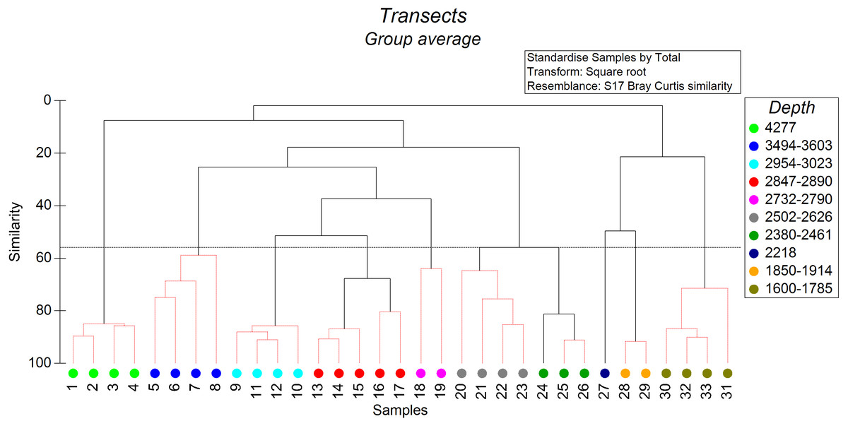
Figure 2: The results of the cluster analysis of soft sediment communities (from quantitative transects) based on the Bray–Curtis similarity index.
The colour indicates the depth range of clustered transects. The black dotted horizontal line corresponds to the 56% similarity level—the level at which the distinct groups of megafauna communities were distinguished. Transects that cannot be significantly differentiated based on SIMPROF tests were connected by red dotted lines (p < 0.05).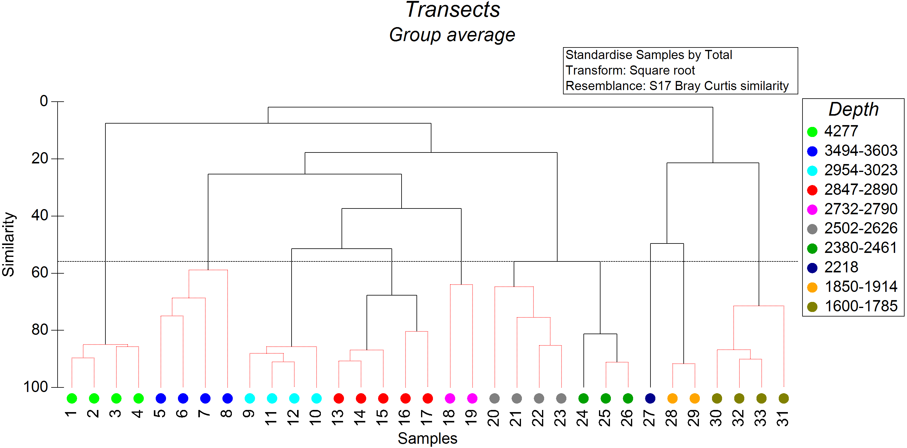
We distinguished separately the depth zone 1,750–1,370 m with 70% hard substrate where sections of the soft and hard substrate were analysed independently. This zone was characterized by frequent occurrence of the sponge Farrea spp on hard substrate (two species of Farrea were collected at similar depths by ROV—F. kurilensis Okada, 1932 and F. aspondyla Reiswig & Stone, 2013) whereas communities of soft substrate were similar to depth zone 1,830–1,750 m (dominance of the holothurian Synallactes chuni Augustin, 1908 and ophiuroids).
Additionally, four depth zones were distinguished within the depth range 1,370–350 m (>90% hard substrate) based on video observations of the dominant taxa.
Characteristics of communities in each depth zone (dominant species on the soft substrate and common species on hard and soft substrate) are given in Table 2 (upper and lower boundaries of depth ranges are given with adjusted based on the visual observations of dominance of the habitat-forming taxa in the whole video footage).
| Depth range (m) | Dominant species on soft and/or hard substrate | Soft substrate (%) | Common species on soft substrate | Common species on hard substrate |
|---|---|---|---|---|
| 4,277–4,278 | Kolga kamchatica | 100% | Echiura gen.sp., Munidopsis spp., Zygothuria sp.1, Psychropotes “raripes ”, Astrocles actinodetus, Enteropneusta gen. sp.1 | Demospongiae varia, Hyalonema sp., Crinoidea (unstalked) |
| 3,610–3,450 | Scotoplanes kurilensis | 90 | Holascus sp., Ceriantharia varia, Umbellula sp., Pennatula sp., Munidopsis spp., Kolga kamchatica, Zygothuria sp. 1, Cucumariidae gen sp., Astrocles actinodetus, Enteropneusta gen. sp.1 | Demospongiae varia, Stylaster spp., Crinoidea (stalked and unstalked), Ascidia varia |
| 3,030–2,910 | Ophiura bathybia, Scotoplanes kurilensis | 90 | Ceriantharia varia, Paelopatides solea | Demospongiae varia, Stylaster spp., Brachiopoda varia, Crinoidea (stalked and unstalked), Ascidia varia |
| 2,910–2,790 | Scotoplanes kurilensis, Ophiura bathybia, Crangonidae gen. sp. | 80 | Ceriantharia varia, Paelopatides solea | Demospongiae varia, Rossellidae varia, Stylaster spp., Alcyonacea varia, Ophiocantha spp., Crinoidea (stalked and unstalked), Ascidia varia |
| 2,790–2,650 | Crangonidae gen. sp. | 80 | Paelopatides solea, Ophiura bathybia | Demospongiae varia, Ophiocantha spp., Crinoidea (stalked and unstalked), Ascidia varia |
| 2,650–2,470 | Paelopatides solea, Crangonidae gen. sp. | 80 | Rhopalonematidae gen. sp. | Demospongiae varia, Alcyonacea varia, Astrochele laevis, Crinoidea (stalked and unstalked), Ascidia varia |
| 2,470–2,290 | Paelopatides solea, Crangonidae gen. sp., Rhopalonematidae gen. sp. | 70 | Torquaratoridae gen. sp., Pannychia aff. moseleyi | Demospongiae varia, Alcyonacea varia, Brachiopoda varia, Ophiura spp., Ophiacantha spp., Crinoidea (unstalked), Ascidia varia |
| 2,290–2,130 | Rhopalonematidae gen. sp., Torquaratoridae gen. sp. | 60 | Paelopatides solea, Pannychia aff. moseleyi, Crangonidae gen. sp. | Demospongiae varia, Rossellidae varia, Alcyonacea varia, Brachiopoda varia, Ophiura spp., Ophiacantha spp., Crinoidea (unstalked), Torquaratoridae gen. sp., Ascidia varia |
| 2,130–1,830 | Torquaratoridae gen. sp. | 50 | Pannychia aff. moseleyi, Synallactes chuni, Ophiura spp., Ophiocantha spp., Rhopalonematidae gen. sp. | Demospongiae varia, Hexactinellida varia, Alcyonacea varia, Brachiopoda varia, Synallactes chuni, Ophiura spp., Ophiacantha spp., Crinoidea (unstalked), Torquaratoridae gen. sp., Ascidia varia |
| 1,830–1,750 | Synallactes chuni, Ophiura spp., Ophiocantha spp. | 40 | Torquaratoridae gen. sp., Ceriantharia varia | Demospongiae varia, Farrea spp., Stylaster spp., Brachiopoda varia, Synallactes chuni, Ophiura spp., Ophiacantha spp., Crinoidea (unstalked), Ascidia varia |
| 1,750–1,370 | Ophiura spp., Ophiocantha spp., Synallactes chuni, Farrea spp. | 30 (stones and dead Farrea) | Torquaratoridae gen. sp., Pannychia aff. moseleyi | Demospongiae varia, Rossellidae varia, Stylaster spp., Paragorgia sp. 1, Munidopsis spp., Galatheidae gen. spp., Lithodidae gen. spp., Brachiopoda varia, Ophiophthalmus sp., Ophiura spp., Ophiacantha spp., Pteraster sp. 2, Goniasteridae gen.sp.2, Hydrasterias sp., Crinoidea (unstalked), Ascidia varia |
| 1,370–720 | Farrea spp., Ophiura spp., Ophiocantha spp. | 10 (stones and dead Farrea) | Ophiura spp., Ophiocantha spp. | Demospongiae varia, Rossellidae varia, Heterochone sp., Heteropolypus ritteri, Paragorgia sp. 1, Munidopsis spp., Galatheidae gen. spp., Lithodidae gen. spp., Psolus spp., Ophiura spp., Ophiacantha spp., Ophiophthalmus sp., Goniasteridae gen. sp. 2 and sp.3, Crinoidea (unstalked), Ascidia varia |
| 720–440 | Heteropolypus ritteri | 0 | – | Demospongiae varia, Farrea spp., Pinulasma fistulosum, Rossellidae varia , Tritonia cf. diomedea, Galatheidae gen. spp., Lithodidae gen. spp., Psolus spp., Goniasteridae gen. sp.2 |
| 440–390 | Heteropolypus ritteri, Corallimorphus pilatus | 0 | – | Demospongiae varia, Caryophylliidae gen. sp. 1, Corallimorphidae gen. sp., Polyplacophora varia, Tritonia cf. diomedea, Terebratulina cf. kiiensis, Goniasteridae gen. sp.2., Solaster sp. |
| 390–350 | Epizoanthus sp. | 0 | – | Demospongiae varia, Actinothoe sp.,Caryophylliidae gen. sp. 1, Corallimorphidae gen. sp., Heteropolypus ritteri, Polyplacophora varia, Terebratulina cf. kiiensis, Ophiopholis cf. japonica, Goniasteridae gen. sp. 2 and sp.3, Pteraster sp. 2, Crossaster papposus |
The dominant taxa changed with depth in the following order: the holothurian Kolga kamchatica Rogacheva, 2012 at the maximum depth (4,277–4,278 m); the holothurian Scotoplanes kurilensis Gebruk, 1983 was dominant or abundant at depths 3,610–2,790 m; the ophiuroid Ophiura bathybia Clark, 1911 sharply dominated at depths 3,030–2,910 m; benthic crangonid shrimps dominated at 2,910–2,290 m with a peak at 2,790–2,470 m; the holothurian Paelopatides solea Baranova, 1955 at 2,650–2,290 m; benthic jellyfish at 2,470–2,130 m; enteropneusts at 2,290–1,830 m; the holothurian Synallactes chuni and ophiuroid of the genera Ophiura and Ophiocantha at 1,830–1,370 m; the glass sponge Farrea spp. at 1,750–1,370 m. At the depths 1,370–720 m almost all benthic epifauna was associated with live or dead colonies of Farrea spp., except of areas of the soft substrate (10% of the total area) dominated by the ophiuroids Ophiura and Ophiocantha. Depths 720–390 m were dominated by the coral Heteropolypus ritteri Nutting, 1909. The corallimorpharian Corallimorphus pilatus Fautin, White & Pearson, 2002 was the dominant at 440–390 m. At the minimum in our study depth 390–350 m, the zoantharian Epizoanthus sp. was the dominant taxon. Contribution to the abundance (in %) per depth zone of the most abundant taxa, based on analysis of quantitative transects, is presented in Fig. 3 and Table 3. Densities of the most abundant taxa are given in Table 3. Characteristic images of all distinguished depth zones with dominant species are presented in Figs. 4 and 5.
Figure 3: The contribution to total abundance (in %) of the most abundant taxa in each of the clustered depth zones.
| Depth range | 4,277–4,278 | 3,610–3,450 | 3,030–2,910 | 2,910–2,790 | 2,790–2,650 | 2,650–2,470 | 2,470–2,290 | 2,290–2,130 | 2,130–1,830 | 1,830–1,750 | 1,750–1,370 |
|---|---|---|---|---|---|---|---|---|---|---|---|
| Kolga kamchatica | 94% | 4% | 0 | 0 | 0 | 0 | 0 | 0 | 0 | 0 | 0 |
| 16.7 ± 8.2 | 0.1 ± 0.2 | 0 | 0 | 0 | 0 | 0 | 0 | 0 | 0 | 0 | |
| Scotoplanes kurilensis | 1% | 32% | 0.7% | 42% | 0 | 0 | 0 | 0 | 0 | 0 | 0 |
| 0.0 ± 0.0 | 1.1 ± 0.9 | 0.8 ± 1.0 | 3.5 ± 3.3 | 0 | 0 | 0 | 0 | 0 | 0 | 0 | |
| Zygothuria sp. | 1% | 12% | 0 | 0 | 0 | 0 | 0 | 0 | 0 | 0 | 0 |
| 0.0 ± 0.0 | 0.3 ± 0.5 | 0 | 0 | 0 | 0 | 0 | 0 | 0 | 0 | 0 | |
| Ceriantharia varia | 0 | 23% | 0.2% | 3% | 19% | 1% | 0 | 0 | 0 | 0.3% | 0 |
| 0 | 0.1 ± 0.3 | 0.2 ± 0.5 | 0.0 ± 0.0 | 0.1 ± 0.3 | 0.0 ± 0,0 | 0 | 0 | 0 | 0.2 ± 0.0 | 0 | |
| Crangonidae gen. sp. | 0 | 4% | 0.05% | 21% | 62% | 69% | 27% | 2% | 0 | 0 | 0 |
| 0 | 0.0 ± 0.0 | 0.0 ± 0.0 | 0.2 ± 0.7 | 0.4 ± 0.5 | 1.1 ± 0.9 | 1.1 ± 1.5 | 0.6 ± 1.1 | 0 | 0 | 0 | |
| Ophiura bathybia | 0 | 0 | 99% | 30% | 10% | 0 | 0 | 0 | 0 | 0 | 0 |
| 0 | 0 | 74.2 ± 24.0 | 3.7 ± 3.1 | 0.2 ± 0.5 | 0 | 0 | 0 | 0 | 0 | 0 | |
| Paelopatides solea | 0 | 0 | 0.05% | 3% | 1% | 21% | 7% | 2% | 0 | 0 | 0 |
| 0 | 0 | 0.0 ± 0.0 | 0.1 ± 0.3 | 0.0 ± 0.0 | 0.5 ± 0.8 | 0.6 ± 0.7 | 0.2 ± 0.4 | 0 | 0 | 0 | |
| Rhopalonematidae gen. sp. | 0 | 0 | 0 | 0 | 0 | 7% | 60% | 53% | 2% | 0 | 0 |
| 0 | 0 | 0 | 0 | 0 | 0.4 ± 0.7 | 3.3 ± 2.7 | 4.2 ± 5.5 | 0,1 ± 0,3 | 0 | 0 | |
| Torquaratoridae gen. sp. | 0 | 0 | 0 | 0 | 0 | 0 | 0 | 44% | 88% | 0.6% | 0 |
| 0 | 0 | 0 | 0 | 0 | 0 | 0 | 8.8 ± 4.1 | 11.9 ± 4.3 | 0.6 ± 0,9 | 0 | |
| Synallactes chuni | 0 | 0 | 0 | 0 | 0 | 0 | 0 | 0 | 3% | 33% | 40% |
| 0 | 0 | 0 | 0 | 0 | 0 | 0 | 0 | 0.5 ± 0.5 | 1.4 ± 1.5 | 0.4 ± 0.5 | |
| Ophiura spp.+Ophiocantha spp. | 0 | 0 | 0 | 0 | 0 | 0 | 0 | 0.05% | 6% | 65% | 58% |
| 0 | 0 | 0 | 0 | 0 | 0 | 0 | 1.1 ± 1.0 | 1.1 ± 1.3 | 3.8 ± 5.9 | 5.2 ± 3.2 |
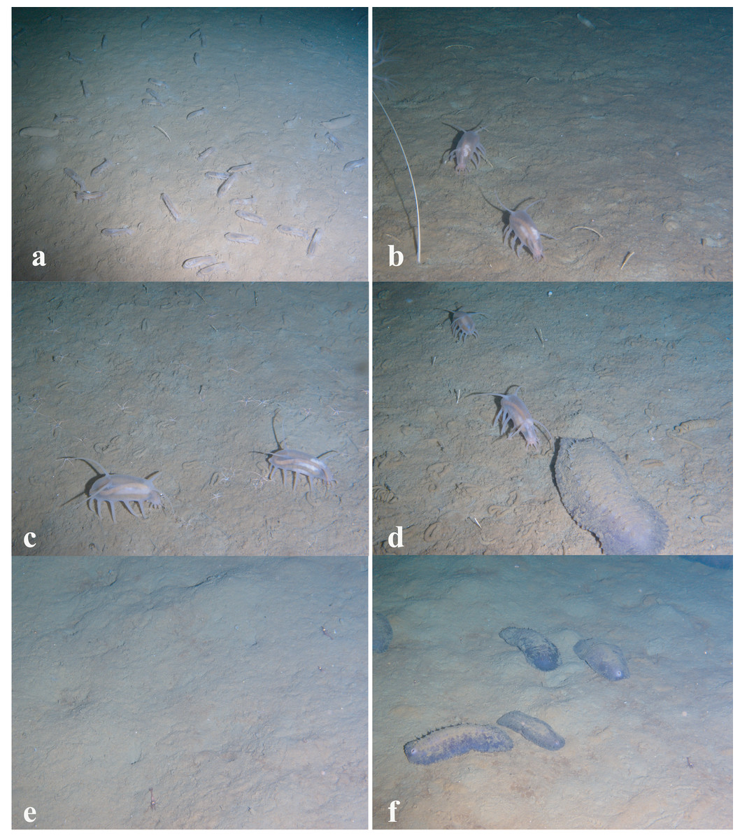
Figure 4: Images of dominant megafauna at different depths.
(A) 4,277–4,278 m, the holothurian Kolga kamchatica. (B) 3,610–3,450 m, the holothurian Scotoplanes kurilensis. (C) 3,030–2,910 m, the ophiuroid Ophiura bathybia and the holothurian S. kurilensis. (D) 2,910–2,790 m, the holothurian S. kurilensis, the ophiuroid O. bathybia and the shrimp Crangonidae gen. sp. (E) 2,790–2,650 m, the shrimp Crangonidae gen.sp. (F) 2,650–2,470 m, the holothurian Paelopatides solea and the shrimp Crangonidae gen. sp.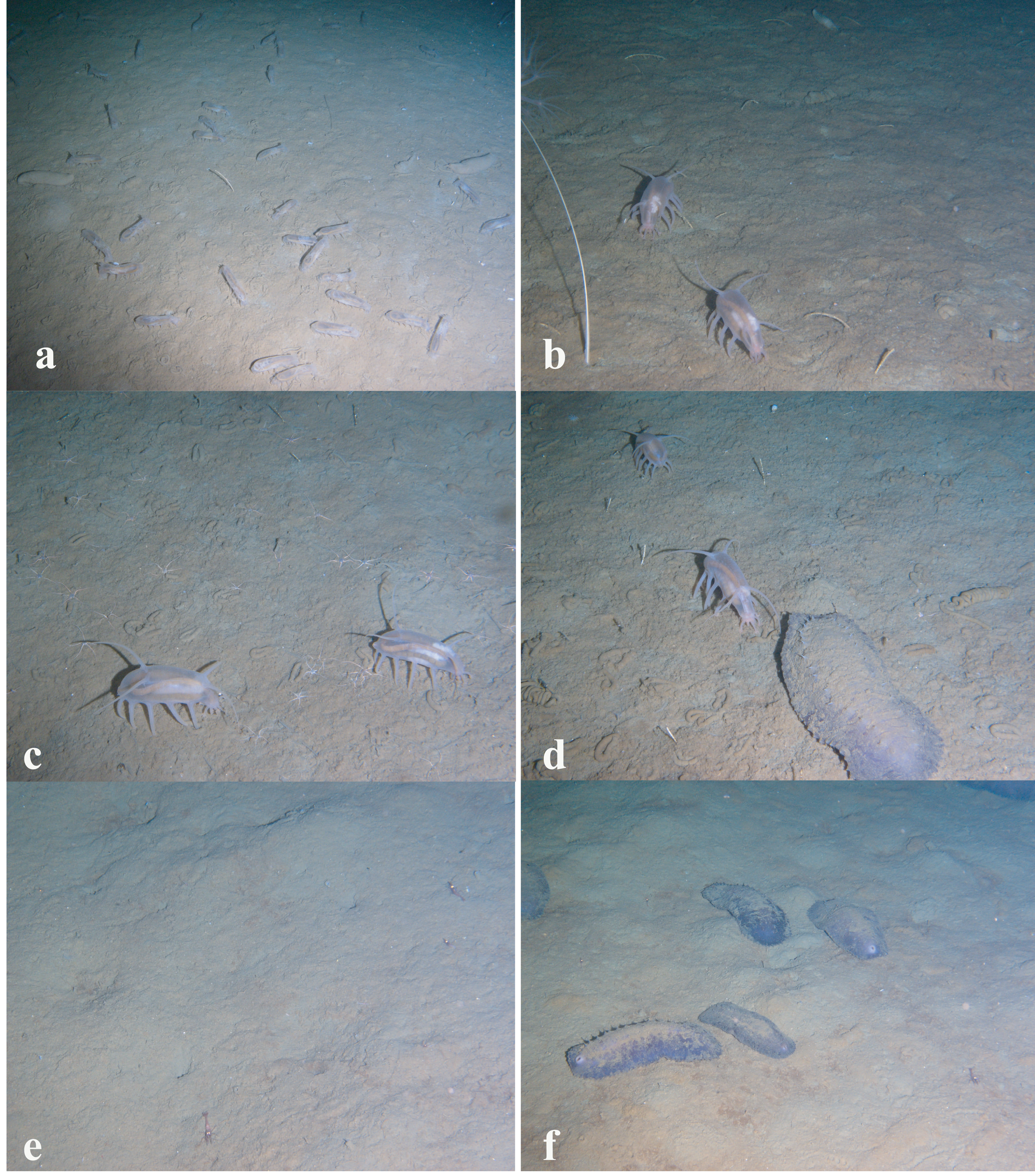
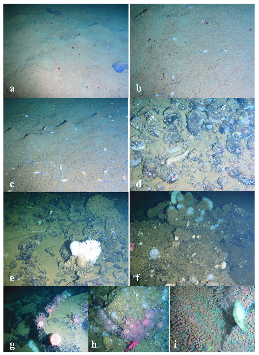
Figure 5: Images of dominant megafauna at different depths (continued).
(A) 2,470–2,290 m, the holothurian Paelopatides solea, the shrimp Crangonidae gen. sp. and the jellyfish Rhopalonematidae gen. sp. (B) 2,290–2,130 m, the jellyfish Rhopalonematidae gen. sp. and the enteropneust Torquaratoridae gen. sp. (C) 2,130–1,830 m, the enteropneust Torquaratoridae gen. sp. (D) 1,830–1,750 m, the holothurian Synallactes chuni and the ophiuroid (Ophiura spp. and Ophiocantha spp.). (E) 1,750–1,370 m, ophiuroids, the holothurian S. chuni and the glass sponge Farrea spp. (F) 1,370–720 m, the sponge Farrea spp. and ophiuroids. (G) 720–440 m, the cnidarian Heteropolypus ritteri. (H) 440–390 m, the cnidarian H. ritteri and Corallimorphus pilatus. (I) 390–350 m, the cnidarian Epizoanthus sp.
The depths with the largest community changes
Based on the vertical distribution of dominant megafaunal taxa, the depths of the largest community changes, or the largest turnover of dominant species, were revealed (Fig. 6). The first pronounced change occurred at ∼2,790 m depth and was identified by the replacement of the holothurian Scotoplanes kurilensis by other species of holothurians, enteropneusts, benthic jellyfish and shrimps. The second pronounced change occurred at ∼1,750 m: here the glass sponge Farrea spp. took the role of the landscape determining species. The third change at ∼720 m was associated with the replacement of glass sponges by soft corals. We also suggest that a community change may have occurred at depths between 3,650–4,200 m (but a lack of observations between 4,277–3,650 m limited more precise zoning). This change was indicated by the replacement of the holothurian Kolga kamchatica by the holothurian Scotoplanes kurilensis.
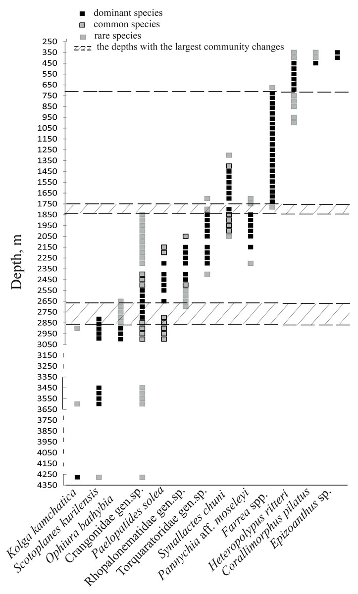
Figure 6: The bathymetric distribution of the dominant megafaunal species.
Each symbol corresponds to the occurrence of a species at a certain depth based on video. The three types of markers show the species status according to the following scale: “dominant”—was more abundant than any other species, “common”—occurred often and was relatively abundant and “rare”—was only met a few times). The dotted lines show the depths with the largest megafauna community changes (the depths of the largest turnover of dominant taxa).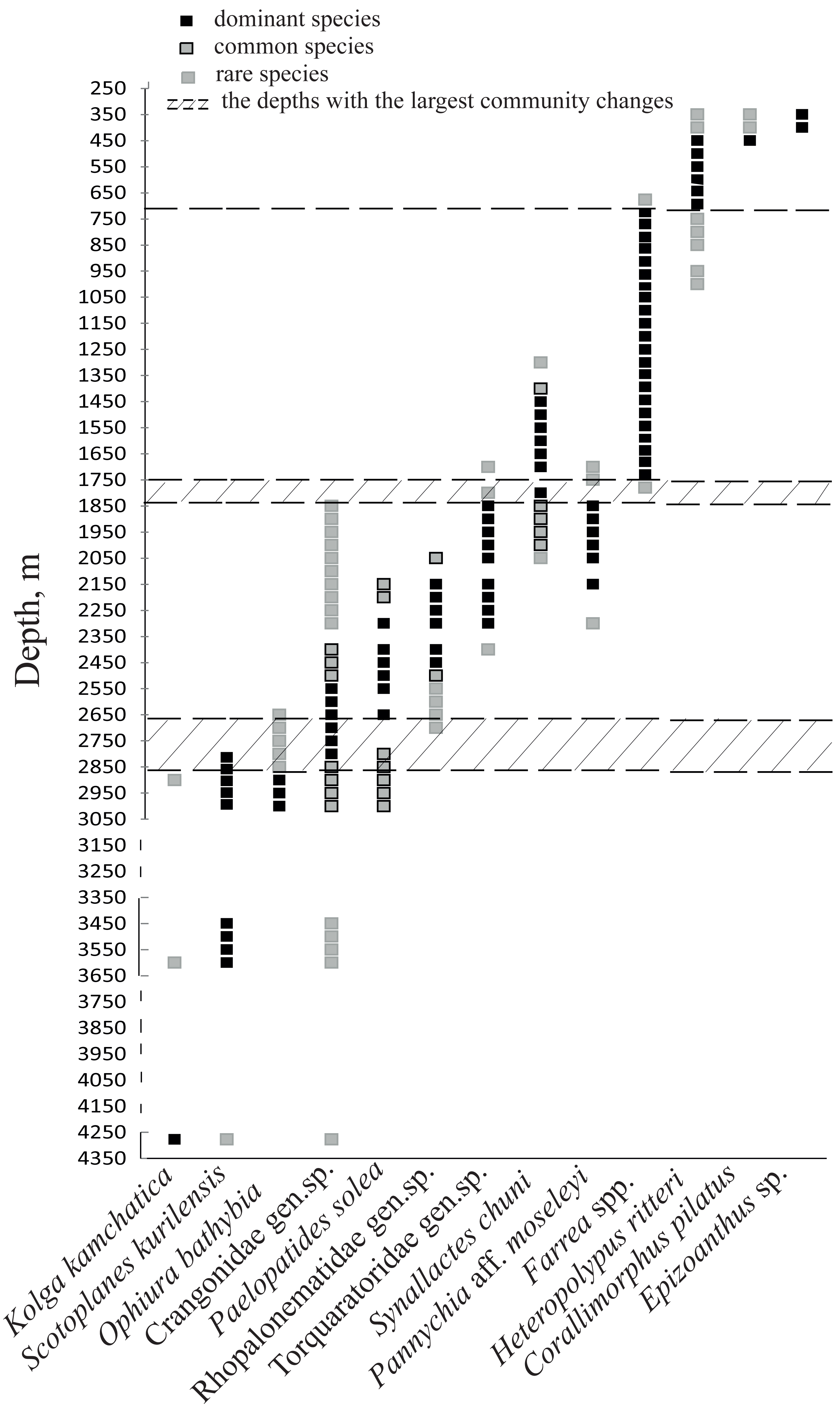
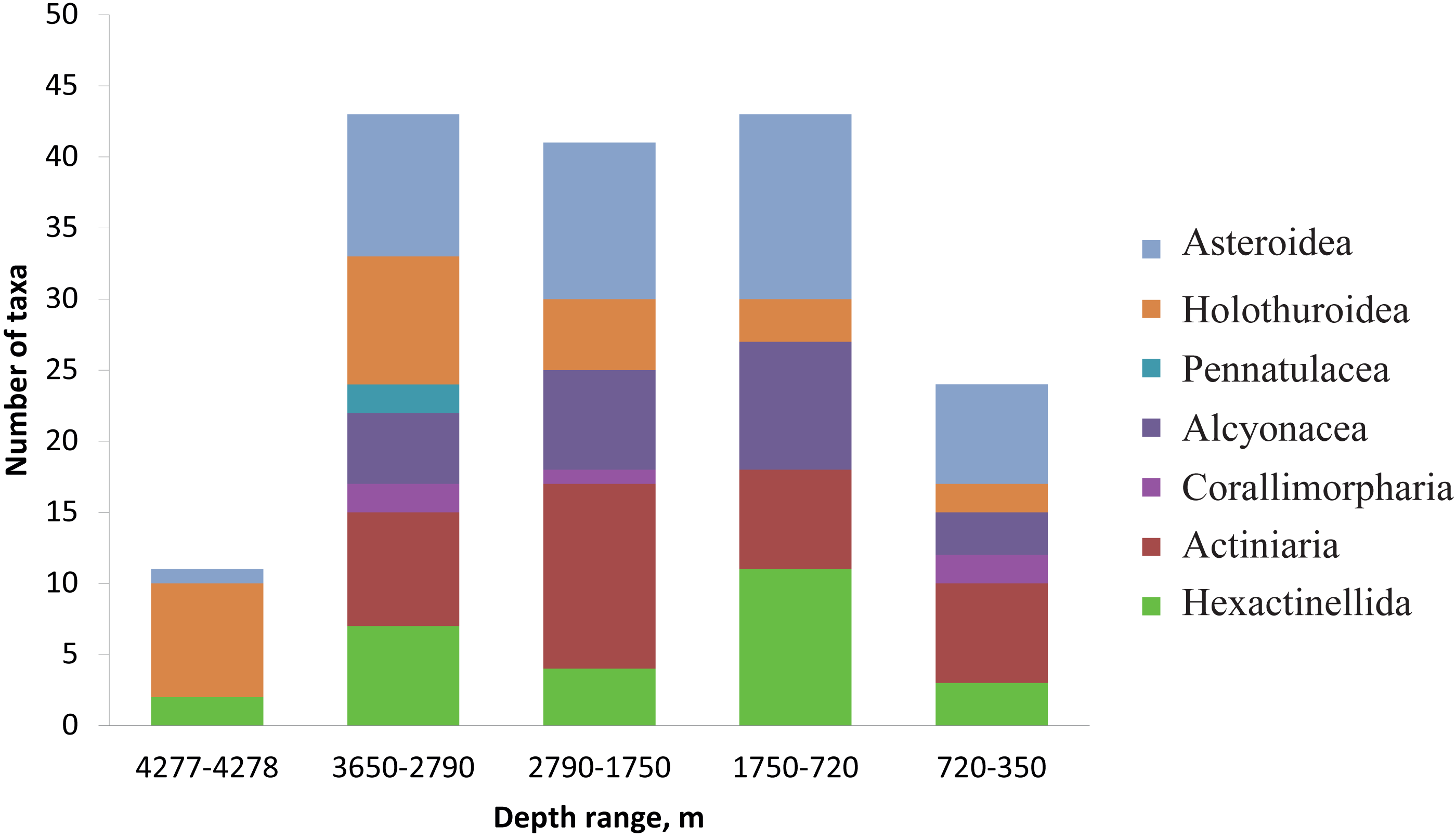
The number of identified species, aggregated into several major taxonomic groups, that occur between depths with the largest community changes is presented in Fig. 7. The highest number of species was found at depths 3,650–2,790 m, the lowest—at 4,277–4,278 m. The taxon with the highest species richness at the maximum depth 4,277–4,278 m was Holothuroidea (eight species). The relatively high number of holothurian species was also at 3,650–2,790 m (nine species). The Order Pennatulacea was recorded only at 3,650–2,790 m (two species). The highest diversity of actiniarians was at depths 2,790–1,750 m (14 species). Alcyonacean corals showed the highest species richness at 1,750–720 m (not less than 9 species). The highest species richness of hexactinellid sponges was at 1,750–720 m (not less than ten species).

Figure 7: The number of identified species, aggregated into several major taxonomic groups, that occur between depths with the largest community changes.
Discussion
In the present study, the vertical distribution of benthic megafaunal communities was described quantitatively for the first time on the slope of the Volcanologists Massif, in the south-west Bering Sea and adjacent Komandorsky Basin in the depth range 4,278–349 m. We were able to identify approximately 170 species, based on the photo and video surveys together with samples taken by ROV. Fifteen depth zones were revealed. Seven species collected using ROV appeared new to science and will be described separately. In addition, three species are assumed to be new to science based on images and/or video records, but further research and sampling using ROV in this area are required for taxonomic clarification.
Soft sediment communities
The greatest depths of the Komandorsky Basin (4,278 m) were dominated by holothurians (eight species) with the prevailing of the elpidiid Kolga kamchatica. Aggregations of small elpidiid holothurians Kolga in the abyssal zone is a phenomenon observed in several areas of the ocean. For example, Kolga nana Théel, 1879 aggregations were found in the Charlie-Gibbs Fracture Zone (Gebruk & Krylova, 2013) with densities of up to 76 ind/m2 and in the Porcupine Seabight in the North Atlantic (Billett & Hansen, 1982) with a mean density of 34 ind/m2 at depths at around 4,000 m. Specimens of K. nana were observed in the Charlie-Gibbs Fracture Zone feeding on the soft sediment mainly in flat and gentle slope areas (Rogacheva, 2012). Another species of this genus, K. hyalina Danielssen & Koren, 1879, was abundant in the Central Arctic Basins with densities significantly dependent on seasonal ice-algae supply to the seafloor (Rybakova et al., 2019). The density of K. kamchatica in our study (17 ind/m2) was lower than in the mentioned reports, although it was still relatively high. Another elpidiid holothurian, Scotoplanes kurilensis, with lower mean density 1–4 ind/m2, was abundant at depths 3,610–2,790 m. In general, elpidiid holothurians can reach high abundances, especially in seafloor depressions in the abyssal zone. Rowe (1971) regarded aggregations of elpidiid holothurians as a typical feature of canyons which trap organic matter that attracts deposit-feeders. However, aggregations of elpidiid holothurians are not exclusive to seafloor depressions: small elpidiids commonly aggregate in areas of accumulation of organic matter on the seafloor (Gebruk, 1990; Billett, 1991; Roberts et al., 2000; Gebruk et al., 2013). Amaro et al. (2010) showed on the example of infaunal molpadiid holothurian Molpadia musculus Risso, 1826 from the Nazare Canyon (NE Atlantic) the key functional role of holothurians in the degradation of organic matter from the sediments and its redistribution and availability for other fauna.
Generally, depths greater 3,500 m in our study were characterized by a high diversity of holothurians (11 species), with one species usually dominant at any given depth. Deposit-feeding holothurians are known to have different feeding strategies and activity (Roberts et al., 2000). Feeding-guilds and niche separation optimize the use of food resources. Studies in various regions showed that holothurians, especially elpidiids, are able to react rapidly to the changes in food supply (Billett et al., 2001; Billet et al., 2010; Gutt et al., 2011; Kuhnz et al., 2014; Huffard et al., 2016).
At 3,610–3,450 m depth, a high diversity of suspension feeders associated with soft substrate was notable, including the hexactinellid sponge Holascus sp., some unidentified species of ceriantharians and two species of Pennatulacea. It can be suggested that this is related to peculiarities of near-bottom hydrodynamics in this area. The growth of the relative importance of sessile suspension feeders (sponges and ceriantharians) deeper than 3,000 m was mentioned by Kuznetzov (1964) based on limited data from the Central and Komandorsky Basins of the Bering Sea: these species developed specific adaptations to the soft-clay habitats, such as raising their bodies above the sediment and the ability to utilize food from the near bottom water layers.
The ophiuroid Ophiura bathybia formed aggregations at 3,030–2,910 m depth with a very high mean density (74 ind/m2). Many ophiuroid taxa are predators (Warner, 1982). Perhaps local sedimentation or hydrological conditions may affect food concentration for them in this area.
At 2,790–2,650 m depth the species diversity and abundance of megafauna were low. Unidentified shrimps of the family Crangonidae were the most notable and abundant soft-sediment megafauna. The hard substrate together with the rare synallactid holothurians and corals at this depth were covered with a considerable sediment layer. We hypothesize that this was an effect of active re-deposition or rapid sedimentation causing decrease in abundance and diversity of megafauna.
On the lower slope, at depths from 3,000 m to 2,150 m, the synallactid holothurian, Paelopatides solea, played a significant role. Numerically they were not dominant, however owing to big size, their contribution to the biomass must have been significant. It means that they may play an important role in ecosystem functioning at that depth range utilizing organic matter from the sediment.
Communities with numerical dominance of benthopelagic rhopalonematid jellyfish at depths >1,500 m (2,470–2,130 m in the present study) to our knowledge have not been reported before. Traditional methods of benthos investigations (trawls and grabs) do not allow the detection of aggregations of gelatinous organisms at the seafloor, because such organisms are usually destroyed in catches. Visual seafloor inspection can resolve this problem. Different observations at depths of up to one and a half thousand meters suggest that deep-sea medusae can be abundant near the bottom (Larson et al., 1992; Matsumoto, Baxter & Chen, 1997; Grange et al., 2017). It can be suggested that aggregations of jellyfish at the seafloor are related to the local near-bottom current regime, apparently increasing food availability through resuspension of organic matter (Larson et al., 1992). Soft sediment megafauna communities dominated by torquaratorid enteropneusts (at the depths 2,130–1,830 m) have not been reported before in the deep-sea either. Deep-sea enteropneusts are also usually gelatinous and easily destroyed in trawl and grab catches. With increased use of ROVs, enteropneusts have been recorded in different deep ocean basins (Priede et al., 2012). Deep-sea enteropneusts are still poorly known, however their function in benthic ecosystems can be important, especially in organic matter processing and surficial bioturbation (Jones et al., 2013). Deep-water enteropneusts feed on the sediment surface, collecting detritus from the substrate, apparently with little or no selectivity as they crawl forward leaving behind a faecal trail of undigestible presumably mineralised material (Holland et al., 2009). Some species have demonstrated the ability to use near-bottom currents to move between feeding grounds in a controlled manner through changes in body posture (Osborn et al., 2012; Jones et al., 2013). Estimation of the area of their traces in the northern part of the Mid-Atlantic Ridge at around 2,500 m depth revealed that enteropneusts contribute significantly to the surficial deposit feeding (Jones et al., 2013). This was unexpected because local deposit feeding megafaunal density was dominated by holothurians, with only a relatively small proportion of enteropneusts (Jones et al., 2013). According to our observations, the mean density of enteropneusts was unusually high reaching 12 ind m−2 at depths 2,130–1,830 m (Priede et al., 2012). The highest density ever previously recorded (for a mixture of Australian torquaratorid species) was 29 worms per 1,000 m2 (Anderson, Przeslawski & Tran, 2011). The highest density found during a 15-year study of Tergivelum baldwinae Holland et al., 2009 from the Pacific Ocean was two worms per 1,000 m2 (Smith, Holland & Ruhl, 2005). In our study area, this taxon definitely must play a major role in the utilization of organic matter at the seafloor.
Small areas of soft sediment (10% of the total area) at depths 1,830–1,370 m were inhabited mainly by the holothurians Synallactes chuni and Pannychia aff. moseleyi Théel, 1882 and some species of ophiuroids. Notably, these species of holothurians and ophiuroids occurred also on hard substrate in that area which may indicate that they are ubiquitous, with no specific adaptations to soft sediment.
Hard substrate communities
The bottom of the Komandorsky Basin was 100% sediment covered, with rare occurrences of colonies of the hexactinellid sponge, Farrea sp. 1, with associated fauna. From the base of the slope up to 1,830 m depth, the area covered by sediment smoothly decreased to 50%, while the area of hard substrate increased. Accordingly, the diversity of species living on rocky outcrops increased, including sessile forms of corals, actiniarians, sponges, ascidians and others. Hard substrate provides more heterogeneous habitat as compared to soft sediment, additionally some organisms use sessile megafaunal species (e.g., sponges, corals) as substrates for attachment (e.g., ophiuroids living on gorgonian corals) (Levin et al., 2001; BuhlMortensen et al., 2010). Some corals and sponges modify habitats through their physical presence. They provide living space, alter physical conditions and affect biological interactions, considerably enhancing diversity (Felley, Vecchione & Wilson, 2008; Miller et al., 2012; Gebruk & Krylova, 2013).
At 1,830 to 1,370 m depth, the area of the hard substrate increased up to 90%. Rocky outcrops alternated with small areas of soft sediment. The deposit feeding holothurians, Synallactes chuni and Pannychia aff. moseleyi, and some species of ophiuroids occurred together with highly diverse sessile suspension feeding fauna on rocks covered by a thin layer of sediment. The ratio of sessile suspension feeders is known to increase on rocks owing to increased active water circulation (Kuznetzov, 1964; Witman & Dayton, 2001; Tyler, 2003; Miller & Etter, 2008; Miller & Etter, 2011). Starting from a depth of 1,750 m, the hard substrates were covered by live and dead colonies of the hexactinellid sponge, Farrea spp., with associated fauna. At 720 m this community was sharply replaced by an assemblage of cnidarians, including Heteropolypus ritteri, Corallimorphus pilatus, Epizoanthus sp. and various actiniarians. From a depth of about 1,750 m, the slope became steeper, possibly affecting water circulation and providing a habitat favourable for suspension feeders. The exact reasons of replacement of sponges by cnidarians remain unknown.
It is important to note that, based on the video or photo images, species could not be equally identified across all taxa, thus limiting the comparison of species diversity at different depths.
Generalized patterns of the vertical zonation
Depths with the largest community changes identified in our study as depths of the largest turnover of dominant taxa, in general correspond to the patterns of vertical zonation recognized by other authors (Carney, Haedrich & Rowe, 1983; Mironov, 1986; Howell, Billett & Tyler, 2002). Major faunal changes occurred at the transition between bathyal and abyssal zones, at ∼2,790 m depth. At this depth, the abyssal community dominated by the deposit-feeding holothurian Scotoplanes was replaced by the bathyal/slope communities of different feeding types (with several dominant species characterized by different feeding types) that may reflect changes in the quality and quantity of food resources at the bottom. The boundary between the abyssal and bathyal zones at a depth of ∼3,000 m was commonly noticed in previous works, however some authors recognized this boundary closer to 2,000 m (Gage & Tyler, 1991) or 4,000 m (Thurman, 1985). In the scheme of the vertical zonation suggested by Belyaev et al. (1959), the bathyal is defined as a depth zone between 200 m and 3,000 m, with a zone between 2,500 m and 3,500 m considered as the transition between the bathyal and abyssal zones. The boundary between the abyssal and bathyal zones can vary around the world based among other factors on geomorphological features of the seabed (Menzies, George & Rowe, 1973). Also, the depth at which this boundary stands out significantly depends on the methodology used. Within the abyssal zone we also identified considerable community change between the Scotoplanes dominated and Kolga dominated communities at depths between 3,650 m and 4,277 m.
The zoning of the bathyal zone also differs in published literature. Many authors distinguish the lower, middle and upper bathyal/slope based on the distribution of species or communities, however the depth boundaries of these horizons differ (Howell, Billett & Tyler, 2002). In the present study we distinguished a variety of communities dominated by soft or hard substrate fauna and deposit-feeding or suspension-feeding species at depths from ∼2,790 m to ∼1,750 m which may correspond to a lower bathyal zone. The mid bathyal zone we recognized between ∼1,750 m and ∼720 m, dominated by suspension-feeding hexactinellid sponges associated with the increased availability of hard substrate. The upper bathyal zone appeared to occur between ∼720 m and 350 m, dominated by suspension-feeding cnidarians on hard substrate. In distinguishing the sub-zones within the bathyal zone, we followed the approach of Belyaev et al. (1959).
The relatively high species richness in our study occurred between the depths of 3,650–720 compared to depth ranges of 4,277–4,278 m and 720–350 m. The peak in species richness occurs at different depths in different World Ocean regions (Gebruk, Budaeva & King, 2010). Our results are concordant with several other authors who observed a peak at around 1,500–3,000 m (Rex, 1981; Howell, Billett & Tyler, 2002; Rex & Etter, 2010).
Thus, the vertical distribution of megafauna communities on the northern slope of the Volcanologists Massif (in the south-western Bering Sea) based on the video survey was examined for the first time. We revealed a distinct pattern of vertical zonation. Fifteen types of megafaunal communities, corelated with particular depth ranges, were distinguished. The largest community changes occurred at depths of ∼2,790 m, ∼1,750 m and ∼720 m. These depths correspond to transitions from the abyssal to the bathyal zone, and to transitions between the lower, middle and upper bathyal zones, as shown in a range of publications by different authors. Our results contribute towards better understanding of the regional patterns of vertical faunal zonation in the World Ocean.
Supplemental Information
Images of megafauna identified during 75th cruise of the RV Akademik M.A. Lavrentyev on video
Complete list of taxa identified on video and in collected material during 75th cruise of the RV Akademik M.A. Lavrentyev
Taxa identified based on collected material are marked by *.
Abundance of all identified species on hard and soft substrate was evaluated visually based on a four-point: 4 - dominant species, 3 - abundant species, 2 - common species, 1 - rare species.