
Seasonal mouse cadaver microbial study: rupture time and postmortem interval estimation model construction
- Published
- Accepted
- Received
- Academic Editor
- Elliot Lefkowitz
- Subject Areas
- Microbiology, Pathology
- Keywords
- Rupture, PMI estimation, Season, Microbiota, Random Forest
- Copyright
- © 2024 Zhao et al.
- Licence
- This is an open access article distributed under the terms of the Creative Commons Attribution License, which permits using, remixing, and building upon the work non-commercially, as long as it is properly attributed. For attribution, the original author(s), title, publication source (PeerJ) and either DOI or URL of the article must be cited.
- Cite this article
- 2024. Seasonal mouse cadaver microbial study: rupture time and postmortem interval estimation model construction. PeerJ 12:e17932 https://doi.org/10.7717/peerj.17932
Abstract
The estimation of postmortem interval (PMI) has long been a focal point in the field of forensic science. Following the death of an organism, microorganisms exhibit a clock-like proliferation pattern during the course of cadaver decomposition, forming the foundation for utilizing microbiology in PMI estimation. The establishment of PMI estimation models based on datasets from different seasons is of great practical significance. In this experiment, we conducted microbiota sequencing and analysis on gravesoil and mouse intestinal contents collected during both the winter and summer seasons and constructed a PMI estimation model using the Random Forest algorithm. The results showed that the MAE of the gut microbiota model in summer was 0.47 ± 0.26 d, R2 = 0.991, and the MAE of the gravesoil model in winter was 1.04 ± 0.22 d, R2 = 0.998. We propose that, in practical applications, it is advantageous to selectively build PMI estimation models based on seasonal variations. Additionally, through a combination of morphological observations, gravesoil microbiota sequencing results, and soil physicochemical data, we identified the time of cadaveric rupture for mouse cadavers, occurring at around days 24–27 in winter and days 6–9 in summer. This study not only confirms previous research findings but also introduces novel insights, contributing to the foundational knowledge necessary to advance the utilization of microbiota for PMI estimation.
Introduction
The utilization of microbial information relevant to cadavers for the purpose of postmortem interval inference (PMI) has ushered in a novel trajectory within the domain of forensic science (Metcalf et al., 2017; Ziqi et al., 2021). Progressing from cadaver temperature measurement (Brown & Marshall, 1974), bodily fluid analysis (De-Giorgio et al., 2021), and the collection of data on necrophagous insect growth and development (Amendt et al., 2011), to the examination of bio-macromolecular compounds (Peng et al., 2020), the methodologies for estimating PMI are continuously advancing. Nonetheless, inherent limitations such as the constrained temporal range of PMI, restricted applicability conditions, and significant margin of error persist, prompting researchers to actively explore supplementary methodologies. Microorganisms constitute the primary contributors to cadaver decomposition (Carter, Yellowlees & Tibbett, 2007), the temporal alterations within microbial communities accompanying cadaver decomposition have captivated the attention of investigators. The capacity of microbial consortia to respond predictably to environmental fluctuations (Metcalf et al., 2017) affording them a distinct advantage in predictive capacities.
Microbial communities associated with the host and environment, especially the gut microbiota, are observed to undergo synchronized growth and proliferation during the progression of cadaver decomposition, originating from the cecum and disseminating towards the liver, spleen, and various parts of the body (Metcalf et al., 2016; Ziqi et al., 2021). From the body parts involved in the study, the current research on utilizing microbial information from diverse biological samples for PMI estimation primarily encompasses gastrointestinal, skin, scalp, liver, oral, heart, brain, and blood samples (Dong et al., 2019; Javan et al., 2016; Li et al., 2023; Tuomisto et al., 2013). Notably, investigations on the gastrointestinal tract are more abundant, encompassing multiple segmented regions. As the postmortem interval prolongs, a reduction in the relative abundance of the phyla Bacteroidetes and Lactobacillaceae is observed in the proximal colon microbiota of decaying bodies (Hauther et al., 2015). The diversity in the cecal region decreases significantly, whereas microbial abundance increases (DeBruyn & Hauther, 2017). Rat rectal bacterial diversity and richness both exhibit a declining trend (Li et al., 2018). Compared to the gastrointestinal tract, the microbial composition of body surfaces such as the skin and hair may play a more significant role in forensic applications (Neckovic et al., 2021). Research on the microbiota of murine abdominal cavities and the surrounding skin suggests that skin samples can provide additional information for PMI assessment (Metcalf et al., 2013). Moreover, microbial information is particularly informative in the early stages of cadaver decomposition for PMI inference. A comprehensive study indicates that facultative anaerobes dominate in bodies with shorter postmortem intervals, while obligate anaerobes dominate in longer intervals (Can et al., 2014). Although research into microbial-based PMI inference is expanding, it remains considerably distant from practical application, necessitating continued in-depth investigation.
Microbiology has achieved significant breakthroughs propelled by the advancement of artificial intelligence (Arrieta et al., 2020). Machine learning can extract patterns within data, and subsequently utilize these patterns for predicting and decision-making in real-world events (Jordan & Mitchell, 2015). It holds pronounced value in managing the vast data generated from microbial sequencing (Jiang et al., 2022; Zou et al., 2020). The classification analysis finds application in personal identification (Meadow, Altrichter & Green, 2014), cause of death analysis (Highet et al., 2014), and geographical inference (Habtom et al., 2019). The regression analysis holds remarkable significance in estimating time of death. With the aid of machine learning, numerous PMI prediction models have been established, such as the PMI prediction model based on bacterial communities within the cecum of rats, exhibiting accuracies of 90.48% for the 0–7 days and 9–30 days prediction groups, with average absolute errors (MAEs) of 0.580 days and 3.165 days respectively (Li et al., 2023). Results from predictive models (Random Forest, RF) constructed using microbial samples from the oral cavity and skin of pig cadavers demonstrate an impressive 94.4% concordance between predicted PMI and actual PMI (Pechal et al., 2014). Another study involving diverse machine learning algorithms for predicting microbiome information from various organs of mice indicates that the Artificial Neural Network (ANN) model yields the best results when applied to postmortem microbial datasets from the cecum. The MAE within 24 h is 1.5 ± 0.8 h, while within 15 days, it is 14.5 ± 4.4 h (Liu et al., 2020). The utility of machine learning algorithms has further fortified the applicability of utilizing cadaver microbiome data for PMI inference.
The surrounding soil of a cadaver is also a reservoir of extensive microbial information, and the introduction of decomposition byproducts from the cadaver into its surrounding environment induces alterations in the adjacent microbial communities (Bergmann, Ralebitso-Senior & Thompson, 2014). Previous studies have substantiated that the bacterial succession in soil surrounding buried cadavers exhibits temporal variations in relation to the PMI (Cobaugh, Schaeffer & DeBruyn, 2015). Therefore, on the basis of our previous study (Cui et al., 2023), this study focuses on mice cadavers and the associated burial soil (gravesoil), while also accounting for seasonal factors, employing a Random Forest-based model to construct a PMI inference framework. Moreover, our investigation identifies the time points at which cadaveric rupture occurs during the decomposition process. These findings lay the theoretical foundation for enhancing the utility of cadaver-associated microbiota data in PMI estimation.
Materials & Methods
Mice model preparation and samples collection
The experimental procedure, animal use and protocols involved in this study have been approved by the Ethics Committee of Central South University (No.2020KT-36). A total of 65 specific pathogen-free (SPF) mice were used for winter experiments, and 45 mice were used for summer experiments. The experimental mice (a total of 110) were provided by Nanjing Qinglongshan Animal Breeding Farm, with an average weight of approximately 20 g per mouse. The mice were sacrificed by cervical dislocation, and corpses were placed in pre-dug pits within the forest located at the Zhongshan Mausoleum in Nanjing, China (32°04′N, 118°50′E). The square plastic containers were placed upside down over the carcasses and buried with about 10 cm of soil. No other processing steps were performed.
Sampling was conducted during winter at days 0, 3, 6, 9, 12, 15, 18, 21, 24, 27, 30, 33, and 36, and during summer at days 0, 3, 6, 9, 12, 15, 18, 21, and 24. At each time point, the contents of the complete intestinal tract of 5 mice were extracted and rapidly frozen in liquid nitrogen, and stored at −80 °C. The gravesoil were divided into two portions: one was stored at −80 °C for microbial analysis, and the other was air-dried for soil physicochemical property testing. As a control, soil from a location 10 m away from the burial site was also collected. The soil temperature (°C) and relative humidity (%) were measured in situ using a soil tester (TA8672, TASI, China). The chemical parameters of soil samples, including total carbon (TC, mg/Kg) content, total nitrogen (TN, mg/Kg) content, pH, and ammonium content, were determined using an elemental analyzer (multi EA 5000, Analytik Jena AG, Germany), flow analyzer (Seal AutoAnalyzer AA3; SEAL Analytical, Germany), and pH meter (PB-10; Sartorious, Germany).
DNA extraction, high-throughput sequencing and amplicon data preprocessing
Total DNA from intestinal contents and gravesoil was extracted using the Soil FastDNA™ Spin Kit (MP Biomedicals, Santa Ana, CA, USA). As a template, the V3-V4 region of the 16S rRNA gene was PCR-amplified using primers with barcodes. The amplification primers used were 341F (5′-CCTACGGGNGGCWGCAG-3′) and 806R (5′-GGACTACHVGGGTWTCTAAT-3′). Amplicons were detected and purified on a 2% agarose gel using the AxyPrep DNA Gel Extraction Kit (Axygen Biosciences, Union City, CA, USA), specifically isolating fragments within the 400–500 bp range. The TruSeq® Nano DNA LT Library Preparation Kit (Illumina, San Diego, CA, USA) was employed to generate sequencing libraries. Library quality was assessed using the Quant-iT PicoGreen dsDNA Assay Kit (Thermo Fisher Scientific, Waltham, MA, USA) and the Agilent Bioanalyzer 2100 System (Agilent, Santa Clara, CA, USA). Sequencing was performed on the Illumina MiSeq PE300 platform (Illumina), yielding raw data.
The “fastq_mergepairs” command from VSEARCH (Rognes et al., 2016) was employed for merging paired-end sequences and subsequently renaming each sequence according to its corresponding sample. Primer sequences and lengths were determined, and sample barcode sequences were extracted. The “fastx_filter” command was utilized to trim primer sequences and barcodes from both ends, ensuring a quality control error rate of <1%. The “derep_fulllength” command was applied to eliminate redundancy in the sequences, resulting in a reduction of data volume by at least one order of magnitude to alleviate downstream analytical burden. Following 97% clustering using USEARCH (Edgar, 2010), representative sequences, either the most abundant or the centroids, were selected as the output. The generation of an OTU feature table was accomplished through the “usearch_global” command in VSEARCH, and taxonomic annotation was performed using the SILVA database (version 123).
The raw data have been uploaded to the NCBI BioProject under the number PRJNA893350.
Data analysis
The α-diversity index is employed for assessing the species richness and evenness of samples. The adequacy of sequencing data is evaluated through the rarefaction curve; a flattening curve indicates reasonable sequencing depth. In the context of β-diversity analysis, NMDS (Non-metric multidimensional scaling) is employed to investigate compositional differences in microbial communities among various samples (Rivas et al., 2013). An optimal result is achieved when Stress <0.1, with values closer to 0 indicating better fit. PERMANOVA (Permutational multivariate analysis of variance) is employed to assess the goodness of fit of different grouping factors to sample dissimilarities, employing permutation tests for statistical significance (Anderson, 2005). The F. Model represents the F-test statistic, R2 indicates the proportion of sample dissimilarity explained by different groupings, with larger R2 values indicating higher explanatory power of groupings, while Pr denotes the P-value obtained from permutation tests; smaller P-values signify greater inter-group disparity significance. A P < 0.05 signifies high confidence in the reliability of the analysis. The taxonomic distribution of samples at various hierarchical levels is presented using a stacked bar plot.
Using GraphPad Prism v9.0 to visualize the changes of the labeled bacteria of the rupture and soil physicochemical factors over time. RDA (Redundancy Analysis) is a form of ordination analysis used to explore the impact of environmental factors on the structure of biological communities (Franklin et al., 2006). RDA seeks a projection that maximizes the variance of response variables while simultaneously retaining the most information from predictor variables.
Analysis tools encompassed the R software’s vegan, dplyr, and ggplot2 packages.
Random forests and PMI estimation
The analysis of microbiome datasets using the Random Forest model has been demonstrated to possess high robustness and superior accuracy (Belk et al., 2018). Regression analyses of microbial sequencing data were conducted using the Random Forest package in the R language to establish PMI inference models for both murine gut microbiota and soil microbiota. Initially, regression analyses were performed on sample datasets derived from different anatomical locations during winter and summer seasons at six taxonomic levels: phylum, class, order, family, genus, and species. The goodness of fit in the regression results was comprehensively assessed to identify the most suitable dataset for model establishment through training. Subsequently, ten-fold cross-validation was employed to select marker species, ranked based on their contributions, and represented through heatmaps. Model evaluation was carried out using correlation coefficients (R2) and Mean Absolute Error (MAE). A high value of R2 should be closer to 1, indicating a stronger predictive performance of the model. A smaller value of MAE signifies greater accuracy in the model’s predictions.
Results
Mouse cadaver decomposition progression
Figure 1 shows the cadaver changes during decomposition of mouse cadavers. In the winter season, the experimental period for mice lasted for 36 days. In comparison to the mice on day 24, which exhibited swelling, there was a noticeable collapse in the cadavers by day 27, becoming even more pronounced by day 30. During the summer experiments, which spanned 24 days, there was a significant and apparent cadaveric decomposition and swelling on day 6, followed by a collapse on day 9, culminating in extensive cadaveric decomposition beyond day 12. These observations suggest that the mouse cadavers between days 24 and 27 during winter experiments, as well as between days 6 and 9 during summer experiments, likely underwent a process of rupture. This process may involve alterations in soil microbiota and physicochemical properties.
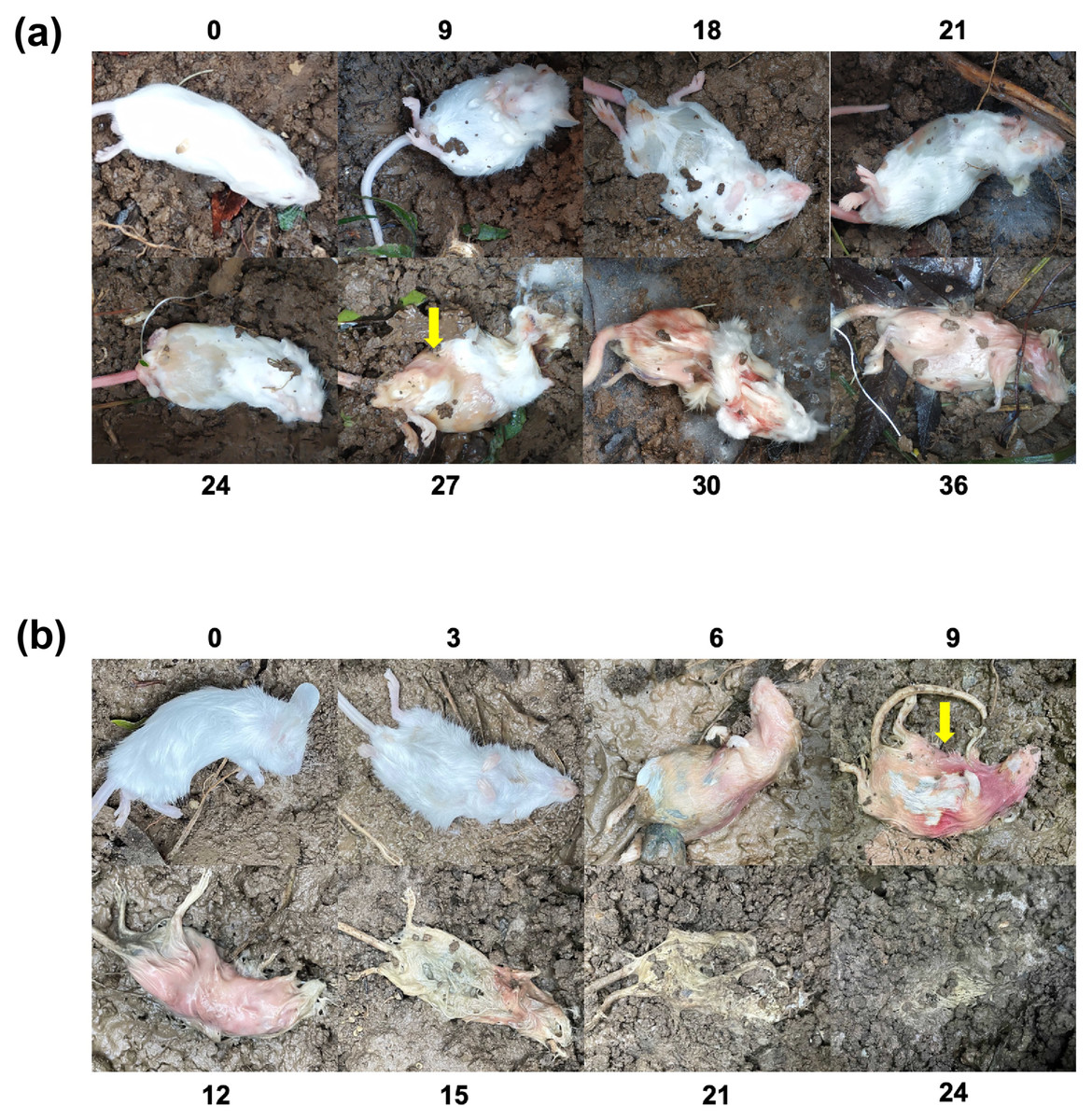
Figure 1: The decomposing process of buried mice.
(A) The winter experiment (36 days). (B) The summer experiment (24 days). The yellow arrow indicates where the body collapsed.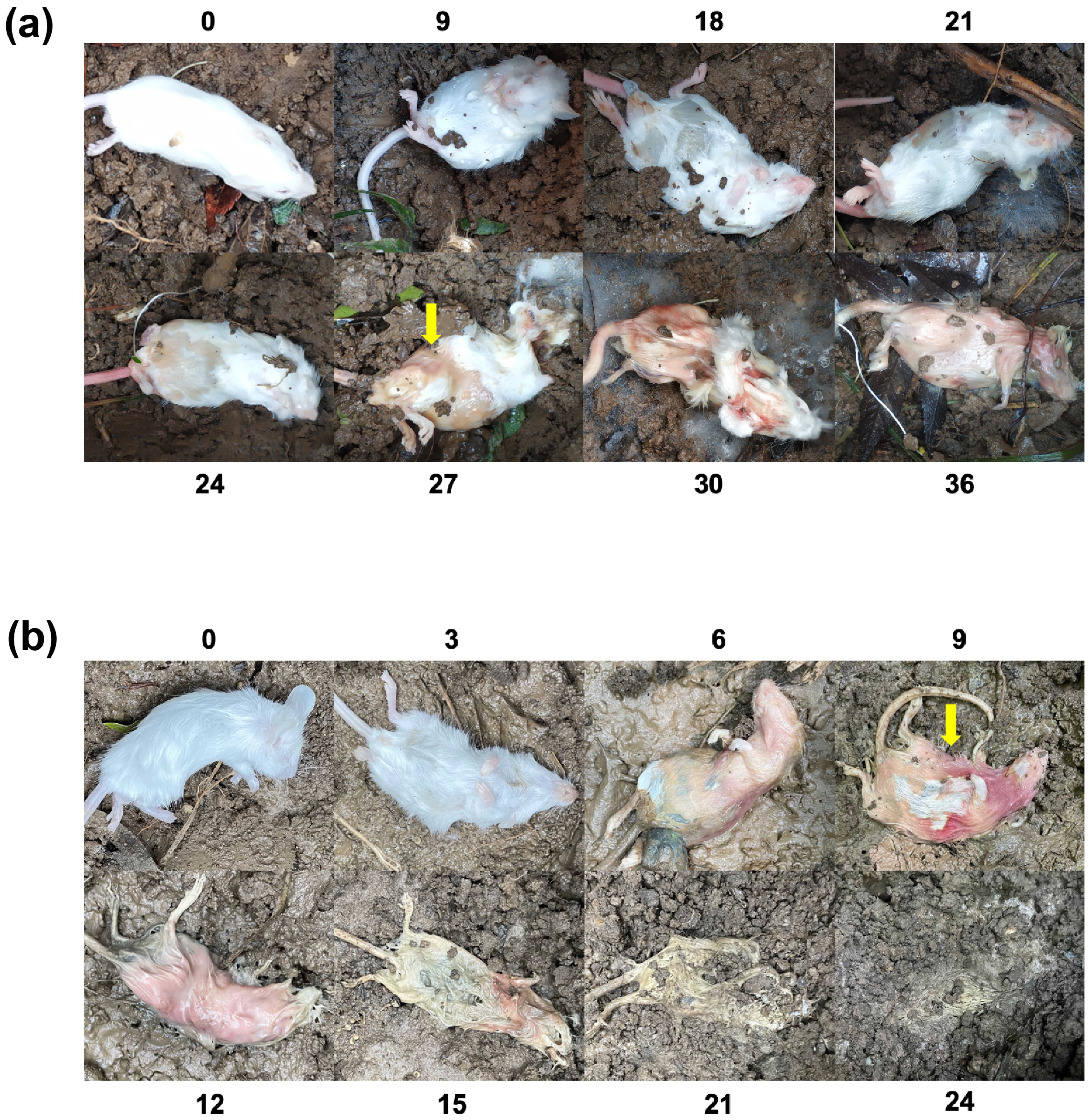
Overview of sequencing results and community structure
A total of 210 samples were collected, comprising 130 winter samples (comprising 65 intestinal content and 65 gravesoil samples) and 80 summer samples (consisting of 35 intestinal content and 45 gravesoil samples). Among these, the fifth gravesoil sample from the third day of winter and the first intestinal sample from the twenty-fourth day of winter did not meet the quality control requirements, resulting in a total of 208 samples eligible for sequencing. After performing quality control, redundancy removal, and other preprocessing steps on all obtained raw sequencing sequences, a total of 9,248,772 effective sequences were retained, with an average sequence length of 422 bp, as detailed in Table S1. These sequences were subsequently clustered into 41,856 operational taxonomic units (OTUs), with winter and summer samples containing 24,736 and 17,120 OTUs, respectively. These OTUs, classified at various taxonomic levels, encompassed 48 phyla, 142 classes, 359 orders, 604 families, 1,431 genera, and 2,785 species. The rarefaction curve (Fig. S1) approaches a plateau at the end, indicating that the sequencing data volume was sufficient, and the sequencing depth adequately covered the majority of microbial species. Thus, the acquired sequencing data are deemed suitable for subsequent analyses.
The top 20 species with the highest average abundance are visualized through stacked column charts (Fig. 2). Within gravesoil samples, the phylum Proteobacteria emerged as the predominant taxonomic group, exhibiting an average relative abundance of 42.72% in summer gravesoil samples. Notably, in winter gravesoil, the relative abundance of the Proteobacteria displayed an overall increasing trend with the progression of PMI. In both seasons, the dominant phyla within gut samples were consistently comprised of Firmicutes, Bacteroidota, and Proteobacteria. Due to space limitations, intricate variations at each taxonomic level are not extensively detailed here. From the community structure, it is evident that certain bacterial changes exhibit temporal patterns irrespective of the season, holding potential for estimating PMI. Furthermore, we observed distinct shifts in community structure in winter and summer samples occurring around days 24–27 and days 6–9, respectively.
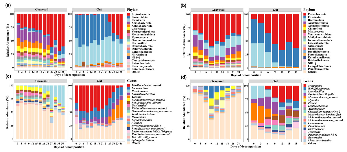
Figure 2: Microbial community structure (Top 20).
(A) and (C) are winter gravesoil samples and intestinal contents samples at phylum level and genus level, respectively. (D) and (E) are summer gravesoil samples and intestinal contents samples at phylum level and genus level, respectively.
Community diversity and potential indicator bacteria for rupture points
The values of alpha diversity indices including Chao1, ACE, Shannon, Simpson, and Inverse Simpson are provided in Table S2. Figs. 3A and 3B depict the changes in Shannon index in gravesoil and intestinal samples during the decomposition of mouse cadavers in winter and summer, respectively. Firstly, regardless of the season, the Shannon index of gravesoil was consistently higher than that of intestinal samples, indicating a higher species diversity in gravesoil. Secondly, for gravesoil samples, significant changes were observed on the 27th day in winter and the 9th day in summer, highlighting significant changes in soil microbial diversity during these two time periods. As for intestinal content samples, although their trends were similar, the values of the Shannon index gradually decreased with time. However, there were no statistically significant differences between adjacent time points in both seasons, indicating that there were no substantial changes in microbial diversity between each sampling point. The NMDS analysis based on Bray-Curtis distances (Fig. 4) demonstrate that both gravesoil and intestinal samples separated distinctly from each other in both winter and summer. Furthermore, the distribution of samples correlated with time. The PERMANOVA results (Table 1) indicate statistically significant differences in the species composition of microbial communities among samples from different locations. The microbial community composition exhibited dynamic changes with PMI, underscoring its potential value in PMI inference.
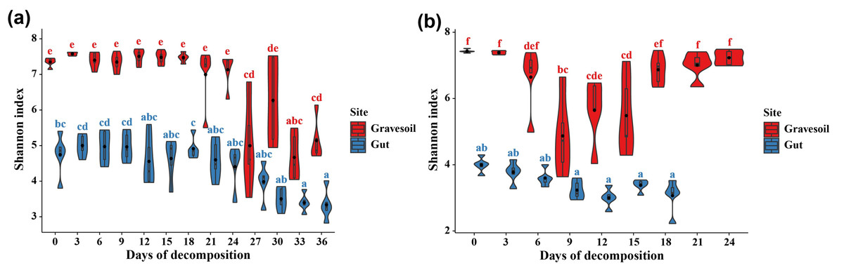
Figure 3: Changes in Shannon index over time.
(A) Winter samples. (B) Summer samples. Gravesoil samples are represented in red and intestinal samples are represented in blue. Using Tukey HSD—multiple comparison test, usually used in the statistical analysis of variance. Its full name is “Tukey’s Honestly Significant Difference” test, with p < 0.05 indicating statistically significant difference and marked using the letter labeling method.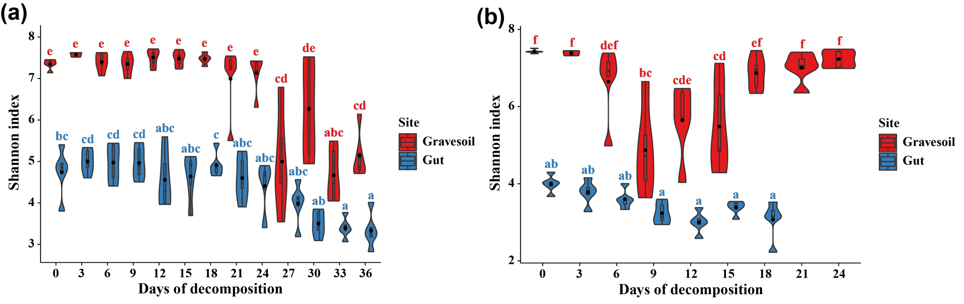
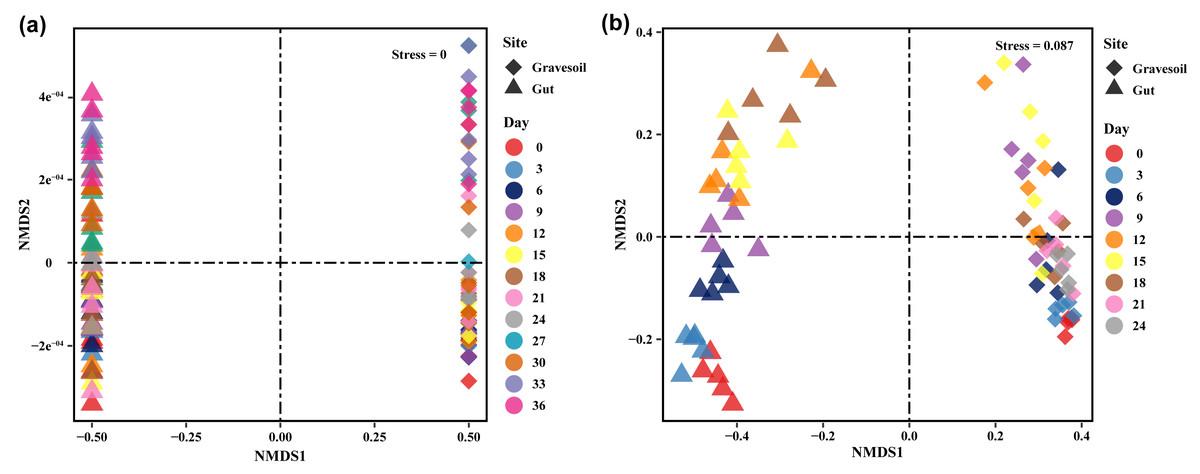
Figure 4: Results of NMDS analysis.
(A) Winter samples. (B) Summer samples. Squares represent gravesoil and triangles represent intestinal contents. Analysis was based on Bray-Curtis distance. Stress < 0.1, indicating better results.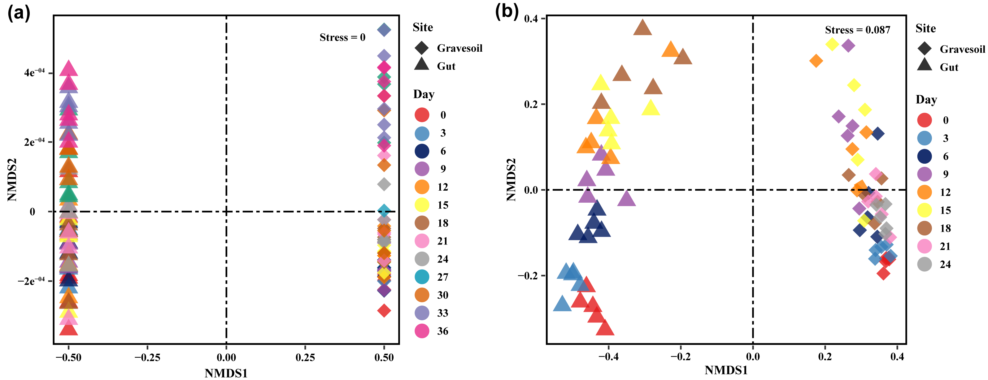
| Season | Compare | F. Model | R2 | Pr (>F) | Sig |
|---|---|---|---|---|---|
| Winter | Gravesoil v.s. Gut | 47.885 | 0.38 | <0.001 | *** |
| Gravesoil ∼ Day | 3.019 | 0.402 | <0.001 | *** | |
| Gut ∼ Day | 4.866 | 0.51 | <0.001 | *** | |
| Summer | Gravesoil vs. Gut | 101.689 | 0.447 | <0.001 | *** |
| Gravesoil ∼ Day | 3.8505 | 0.475 | <0.001 | *** | |
| Gut ∼ Day | 2.806 | 0.398 | <0.001 | *** | |
Notes:
Sig: ***, P ≤ 0.001.
∼ Day, comparison between different decomposition time samples.
Based on our preceding analyses, the microbial community shifts observed around days 24–27 and days 6–9 cannot be overlooked, potentially signifying the time of rupture. However, microbial diversity changes in gut samples across both seasons showed no significant disparities. This phenomenon may be attributed to the relatively closed nature of the gut environment, wherein even if rupture occurs, the gut milieu remains relatively stable. Consequently, this study conducted differential abundance analyses on soil microbiota for the two seasons, aiming to pinpoint bacteria that are not influenced by seasonal variations and may serve as markers for the rupture point. At the phylum level, we identified three candidates, including Gemmatimonadota, Desulfobacterota, and MBNT15. At the genus level, a total of 31 candidates were identified, with four differential bacteria selected from the top 20 differential taxa, namely Desulfobacterota_norank, Steroidobacteraceae_uncultured, Gemmatimonadaceae_uncultured, and Rokubacteriales_norank. The relative abundance fluctuations of these bacteria throughout the decomposition process are visualized in Fig. 5 and Fig. S2. Notably, their relative abundances exhibited significant decreases on day 27 in winter and day 9 in summer, followed by a gradual resurgence in the subsequent time intervals.
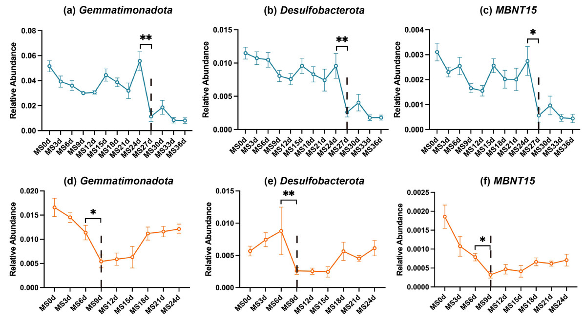
Figure 5: Potential indicator bacteria for rupture points (at the phylum level).
Blue (top row) represents the winter season, while orange (bottom row) represents the summer season. Statistical analysis was performed using the Wilcoxon test; **, P ≤ 0.01; *, P ≤ 0.05.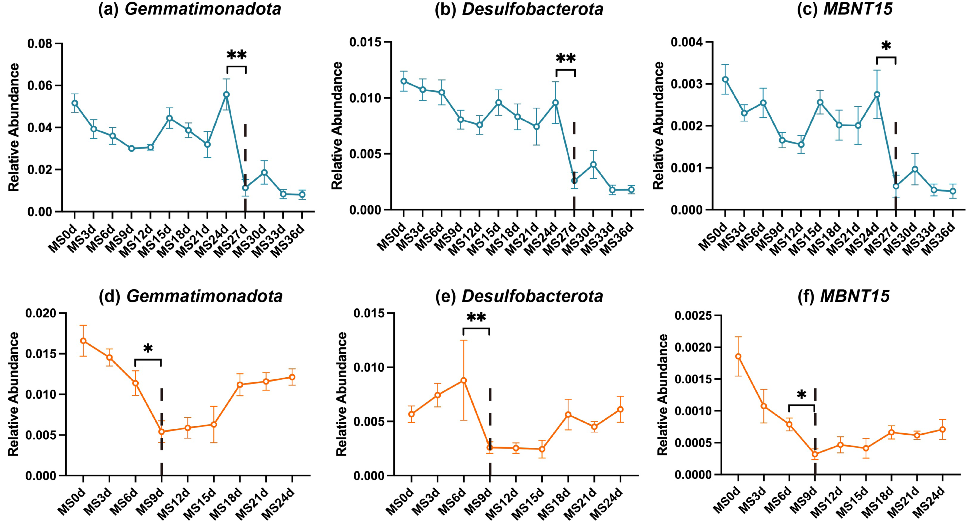
Environmental factor correlation analysis
The alterations in the microbial community structure of gravesoil may be linked to the exchange of substances between cadavers and their surrounding environment resulting from cadaveric rupture. The relationship between the microbial community in the gravesoil and soil physicochemical properties (environmental factors) is depicted in Fig. 6. Regardless of season, temperature, ammonium salts, and pH emerge as the three primary factors influencing the microbial community structure in gravesoil. The microbial community in gravesoil exhibits a negative correlation with both ammonium salts and pH during days 0–24 and days 0–6, while displaying a positive correlation during days 27–36 and days 9–18. This suggests that after day 27 and day 9, the microbial community structure in gravesoil is primarily influenced by changes in ammonium salt content and pH, remaining unaffected by seasonal variations. This also suggests that cadaveric rupture may occur around these two time points. The temperature, predominantly influenced by the season, exerts contrasting effects on these two factors.
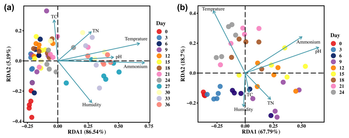
Figure 6: The RDA analysis results.
(A) Winter samples. (B) Summer samples. Arrows represent environmental factors, and the length of the line connecting the arrow to the origin signifies the strength of correlation between an environmental factor and community and species distribution. Longer lines indicate stronger correlations, while shorter lines suggest weaker correlations. Dots represent sample points, with different colors denoting different days. The angles formed between samples (connected to the origin) and environmental factors illustrate the nature of the correlation (acute angle, positive correlation; obtuse angle, negative correlation; right angle, no correlation).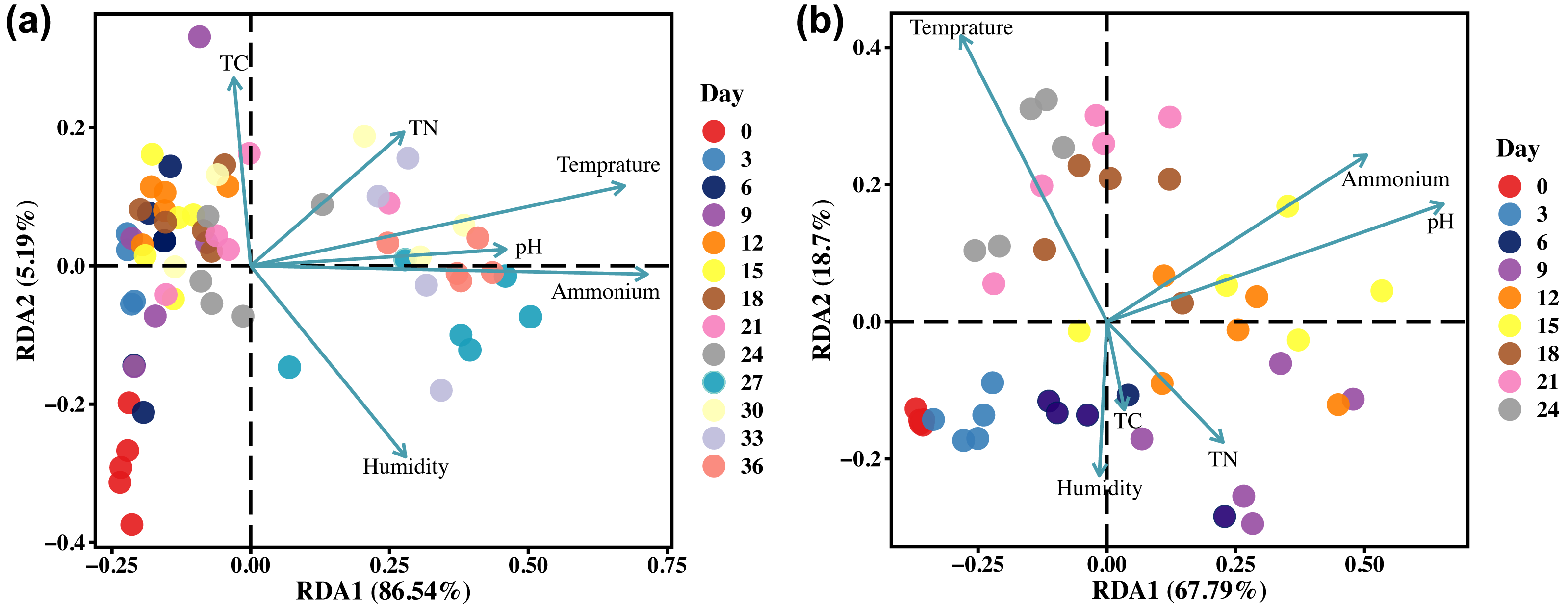
Figure 7 and Fig. S3 are presented to illustrate the trends in these physicochemical properties during the cadaveric decomposition process. Winter temperatures remain below 10 °C, while summer temperatures exceed 16 °C, with no differences observed between gravesoil and control soil. With the progression of cadaveric decomposition, the pH value and ammonium salt content in gravesoil gradually increase compared to the control group, culminating upon completion of cadaver decomposition. This change is particularly pronounced on day 9 of the summer season, aligning with the previously analyzed time points. In contrast, the significant change in the winter season does not occur on day 27; ammonium salt content in winter exhibits significant variation between days 30–33. While there is no statistically significant difference in winter pH changes, there is a noticeable increase on day 30 compared to day 27, maintaining an upward trend until the end of the experiment. This could be attributed to the low winter temperatures, resulting in a slower and delayed cadaveric exudate compared to the more rapid process in summer.
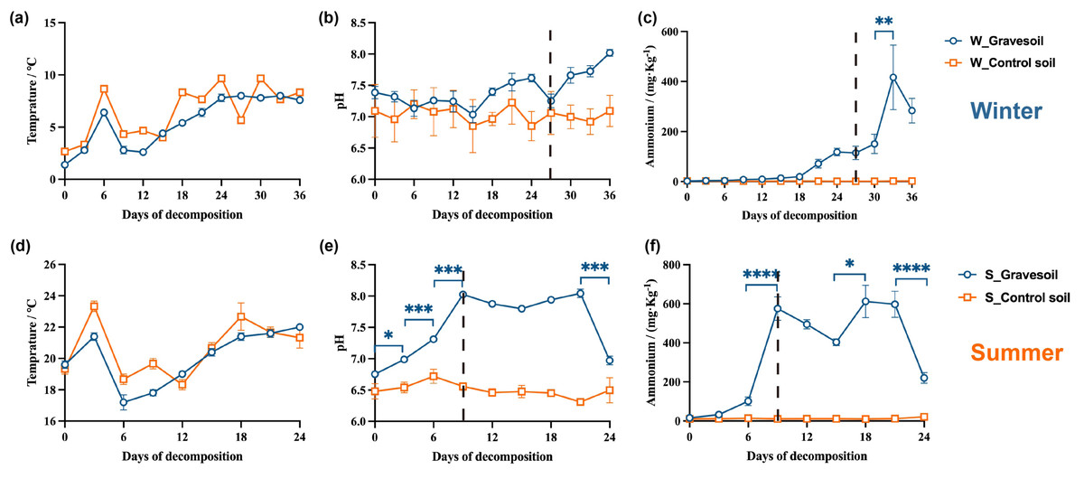
Figure 7: Changes in physicochemical properties of gravesoil.
The first row (A–C) shows the winter experiment and the second row (D–F) shows the summer experiment. Blue circles represent gravesoil samples, and orange squares represent control soil samples. The statistical method was ordinary one-way ANOVA, ****, P ≤ 0.0001; ****, P ≤ 0.001; **, P ≤ 0.01; *, P ≤ 0.05.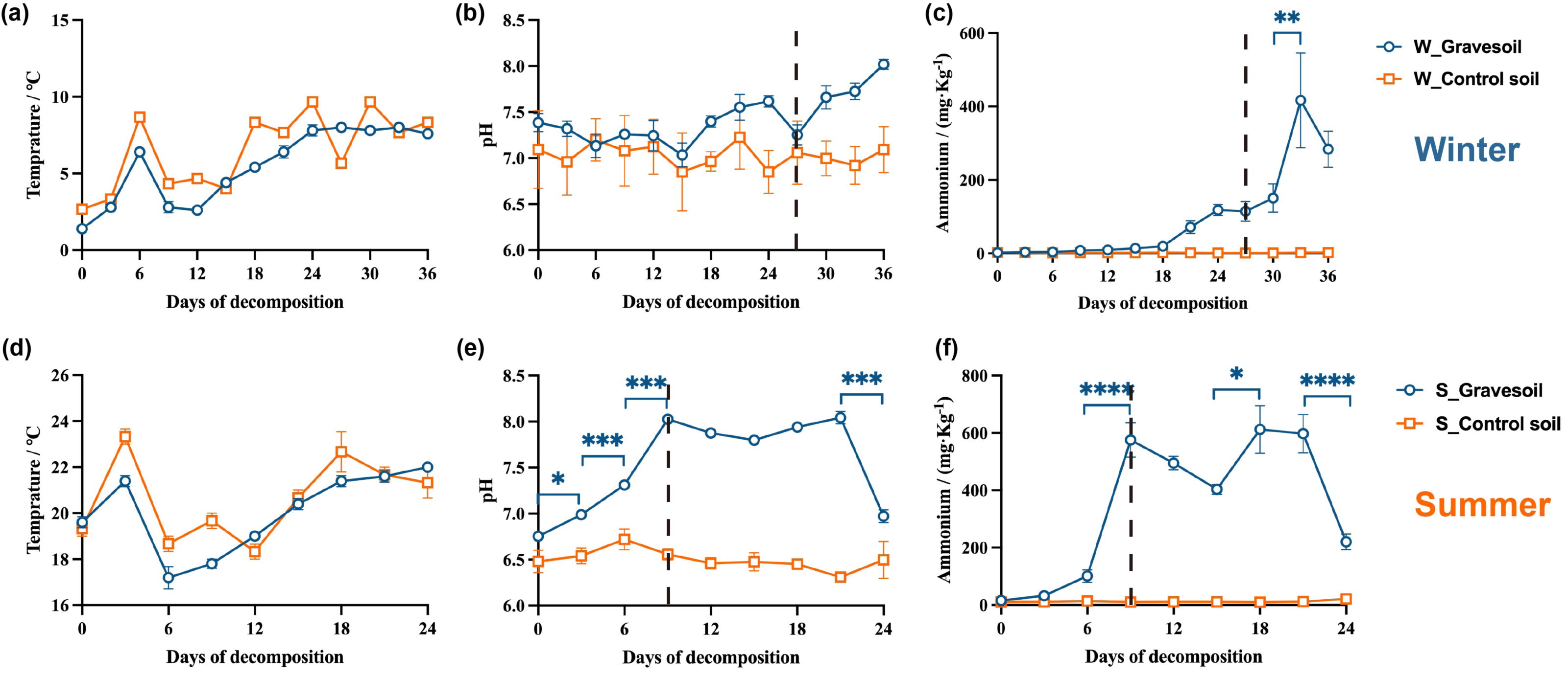
Based on the aforementioned research findings, we propose that cadaveric rupture occurs on day 27 in winter and day 9 in summer. Additionally, regardless of the season, the microbial community in gravesoil undergoes significant changes following rupture, which are closely associated with variations in ammonium salt content and pH in the soil.
PMI estimation model
We constructed PMI inference models for winter gravesoil, winter gut contents, summer gravesoil, and summer gut contents. The goodness of fit reached the highest at the genus and species levels. Considering the prevalence of uncultured species at the species level, we ultimately selected the genus-level dataset for model development. The results of these models are presented in Figs. 8A and 8C and Figs. S4A and S4C.
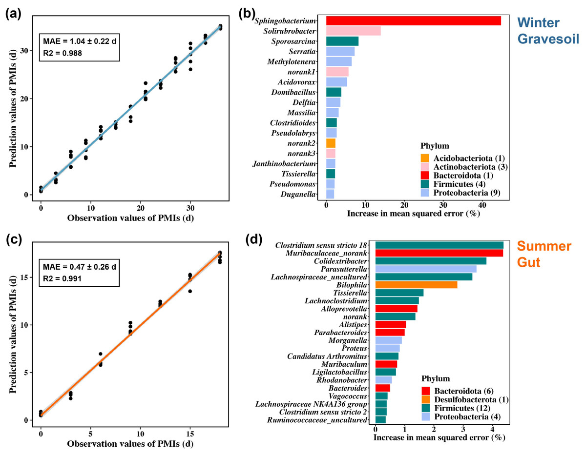
Figure 8: PMI estimation model and corresponding marker microbial taxa. The first row represents the winter sample and the second row represents the summer sample.
(A) and (C) are constructed using gravesoil microbes in winter and gut microbes in summer, respectively. (B) and (D) are the marker bacteria selected by each model, with 18 genera in winter and 23 genera in summer.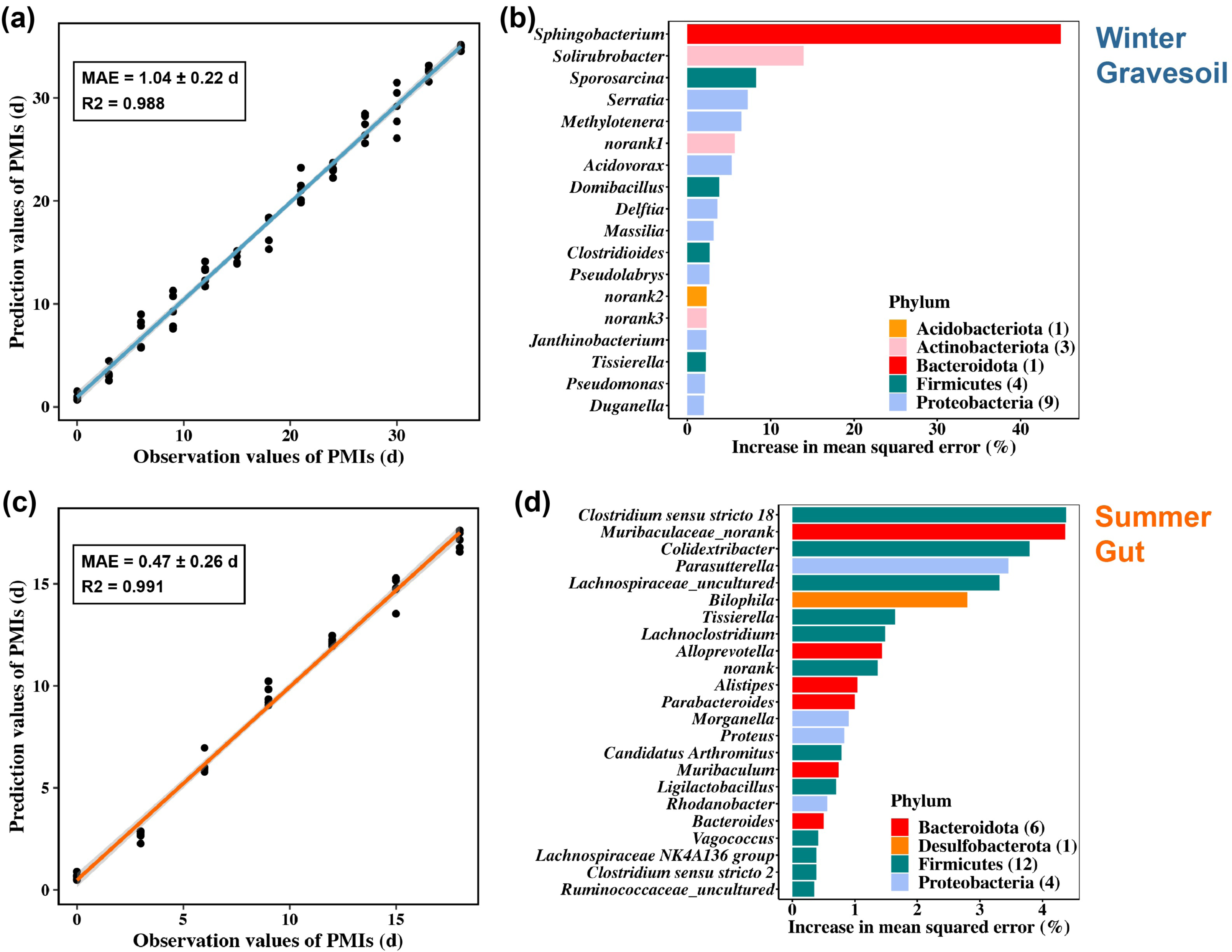
Overall, the summer model exhibits a lower MAE and higher inference accuracy. Specifically, the winter model demonstrates higher accuracy in inferring PMI based on gravesoil microbiota, while the summer model excels in inferring PMI using gut contents microbiota. Furthermore, through a ten-fold cross-validation analysis, 18 PMI-related marker microbial taxa were identified for winter samples, and 23 for summer samples. These taxa were ranked by their importance at the genus level (Figs. 8B and 8D and Figs. S4b and S4d). In winter samples, the most influential genus in gravesoil is Sphingobacterium from the Bacteroidota phylum, with half of the top 18 genera originating from Proteobacteria. In the gut, the most significant genera are Yersinia followed by Pseudomonas, both belonging to Proteobacteria. In summer samples, the most pivotal gravesoil genus is Erysipelothrix from the Firmicutes phylum, with nearly half of the genera belonging to Proteobacteria. In the gut, the essential genera predominantly belong to Bacteroidota and Firmicutes. In summary, phyla Proteobacteria, Bacteroidota, and Firmicutes house key bacteria for PMI inference. Given the varying decomposition periods of mice in different seasons, constructing PMI inference models based on season-specific cadaver microbiota is essential for accurate PMI estimation.
Discussion
There are several reasons hindering the widespread application of microbiology in forensic practice. Apart from the various factors that can influence microbiota themselves, such as age, underlying diseases, and cause of death, the accessibility of human cadavers as research subjects is limited. Additionally, the cost associated with sequencing is also a significant consideration (Speruda et al., 2022; Tozzo et al., 2022). The use of microbiota for PMI estimation is still in its nascent stages and requires further research. In this study, mice were employed as the research subjects with the objective of developing PMI estimation models for two seasons, utilizing microbiota data from both gravesoil and intestinal contents, aided by Random Forest. Throughout this process, in conjunction with the decay process of mouse cadavers and the fluctuation in microbial diversity in the gravesoil, we identified the time points at which cadaver rupture occurred in different seasons. We posit that the occurrence of cadaver rupture led to significant alterations in the microbial community and physicochemical properties of the gravesoil. In the following sections, we will delve into a detailed discussion of these findings.
The decomposition of a cadaver is a gradually evolving process with distinct morphological features including cadaveric odor, green discoloration, and bloating, which can be categorized into the stages of Active Decay (including bloating and rupture) and Advanced Decay (Carter, Yellowlees & Tibbett, 2007; Cong, 2016; Parkinson et al., 2009). The role of microbiota in this process is inseparable. Research by Metcalf et al. (2013) and Hyde et al. (2013) has corroborated Evan’s hypothesis that a significant microbial community transition occurs when cadaveric bloating ceases (Evans, 1963). In this experiment, we first observed bloating and collapse of mouse cadavers, occurring around days 24–27 in winter and days 6–9 in summer. These observations suggest that cadaveric rupture may occur during these periods. Subsequently, the significant changes in the community structure and diversity of gravesoil microbiota at these time points further support our hypothesis.
Microbial activities generate chemical byproducts of decomposition, such as ammonia, hydrogen sulfide, and amines, which alter the physicochemical properties of the soil (Mondor et al., 2012), including an increase in pH (Metcalf et al., 2013). Building upon our previous study (Cui et al., 2023), this research considers two seasons and finds that the timing of increased ammonium content and elevated pH aligns with our expected rupture points, occurring after days 6–9, but with a delayed onset in winter. We attribute this delay to the lower temperature in winter, resulting in reduced enzymatic and microbial activity, which in turn slows down decomposition compared to summer, thus causing a delay in the changes in ammonium content and pH in the soil. In light of this study, we propose that days 24–27 in winter and days 6–9 in summer represent the cadaveric rupture points for mouse cadavers. This aligns with Metcalf et al.’s (2013) findings that cadaver rupture occurs around days 6–9. And they showed in another report that the significant change of ammonium salt and pH in winter and spring was about 30 days, suggesting that the time point of rupture was similar to our results (Metcalf et al., 2016). It is imperative to note that, while the outcomes exhibit similarity, there are disparities in the cadaver handling methods and the specific temperature settings of the experiments. Our study investigated the interment of mouse carcasses within a natural environment, whereas their research entailed exposed mouse carcasses within controlled laboratory conditions. Consequently, further research endeavors are requisite to delve deeper into and substantiate this matter.
Simultaneously, we conducted the selection of indicator bacteria for rupture point. Unlike Metcalf et al. (2013), this study primarily focused on gravesoil bacteria. In this experiment, we found no significant differences in the microbial community near the rupture point in intestinal samples, possibly due to the relatively enclosed and stable nature of the intestinal environment, which minimizes the impact of cadaver rupture. Based on the changes in gravesoil microbiota, the indicator bacteria for rupture point were primarily Gemmatimonadota, Desulfobacterota, and MBNT15 at the phylum level. Gemmatimonadota is widespread in soil, aquatic environments, and sediments, with limited specific studies (Mujakić, Piwosz & Koblížek, 2022; Zeng et al., 2016). Desulfobacterota has been formally classified at the phylum level (Göker & Oren, 2023; Waite et al., 2020) and can participate in organic matter degradation and sulfate reduction processes (Murphy et al., 2021). MBNT15 was discovered during phylogenetic analysis of 16S rRNA gene sequences obtained from paddy soil (Begmatov et al., 2022). Comparative genomic analysis indicates that MBNT15 is distantly related to Desulfobacterota, with the ability to reduce sulfur and nitrogen compounds but not sulfate (Chen et al., 2021). While there is no direct experimental evidence, existing literature suggests that these three phyla are closely associated with the production of cadaveric decomposition products such as ammonia, hydrogen sulfide, and amines.
The relative abundance of these three phyla significantly decreases after cadaveric rupture, followed by gradual recovery. This is likely due to the entry of microbial communities from the soil into the cadaver through the rupture site, causing changes in the relative abundance and diversity of this specific part. This observation does not contradict Metcalf et al.’s (2013) perspective, which posits that the dominant microbial community in the cadaver shifts from intestinal bacteria to environmental bacteria after cadaveric rupture. Regarding the selected differential bacteria, their relative abundance did not significantly increase, possibly because the microbial population in soil is much larger. However, further analysis is required, particularly with regard to microbial communities in mouse cadaver sites in contact with the gravesoil, a component not included in this study. Therefore, these three phyla serve as preliminary candidates for marker bacteria associated with the rupture point from the perspective of gravesoil.
In addition, this study established a PMI estimation model using the Random Forest algorithm based on microbial data. Firstly, in alignment with prior research (DeBruyn & Hauther, 2017; Guo et al., 2016; Liu et al., 2020), Proteobacteria, Bacteroidota, and Firmicutes have been identified as taxonomic phyla of significance for PMI estimation. Secondly, irrespective of season or sample type, microbial succession during the decomposition of cadavers emerges as a predictable temporal metric post-mortem, corroborating the feasibility of microbiota-based PMI estimation, in conjunction with studies like Metcalf et al. (2016).
Our findings indicate superior PMI estimation performance for summer samples, but the collection and analysis of microbiota data from different seasons offer more practical utility. Presently, research in this field encompasses human, mouse, rat, and pig cadavers, with a focus on sample collection sites, modeling algorithms, and community succession discussions (Hauther et al., 2015; Hyde et al., 2013; Javan et al., 2016; Metcalf et al., 2013; Pechal et al., 2014). As the results of Burcham et al. (2024) on human cadaver showed, factors such as climate, geographical location, and season can significantly affect microbial decomposer community ecology. A study involving the burial of rats in a natural environment during the autumn-winter season (September 20th to November 19th) demonstrated that, among three sampled sites (gravesoil, cecum, and skin), the Random Forest algorithm exhibited the best modeling performance using grave soil microbiota data, with a MAE of 1.82 days within the 60-day decomposition period (Zhang et al., 2021). Similarly, our results reveal that, during the winter season (December 29th to February 3rd), gravesoil data also yields the best modeling performance with an MAE of 1.04 days. However, in our summer experiments, the most effective modeling dataset is derived from intestinal contents, with an MAE of 1.04 days. Another study conducted under laboratory conditions at 25 °C suggests that using intestinal data is the most robust approach for PMI estimation (Liu et al., 2020). Although their study population differs slightly from ours, it still provides valuable insights. Based on this analysis, we propose the following recommendations: for winter (low-temperature) cadavers, we recommend prioritizing gravesoil microbiota data for constructing PMI estimation models, while for summer (high-temperature) cadavers, we suggest prioritizing microbiota data from intestinal content for PMI estimation modeling.
Conclusions
In summary, this study provides preliminary evidence for the timing of cadaveric rupture in mice, occurring around days 24–27 in winter and days 6–9 in summer. Following cadaveric rupture, the initially bloated cadaver undergoes a collapse, facilitating the exchange of microbiota between the cadaver and the surrounding soil/grave soil. Decay products, such as ammonium salts, from the cadaver are introduced into the adjacent soil, leading to alterations in the microbial community structure of the gravesoil and concurrent increases in ammonium salt content and pH levels. Based on changes in grave soil microbiota and physicochemical properties, we have tentatively identified three candidate marker bacteria for cadaveric rupture points: Gemmatimonadota, Desulfobacterota, and MBNT15 at the phylum level. This research serves as a foundational contribution to the limited body of literature on cadaveric rupture and its microbial implications, facilitating future segmented post-mortem interval estimations using this knowledge. Moreover, based on the results of the PMI estimation models established by Random Forest, we recommend employing gravesoil microbiota data for PMI estimation models in winter (low-temperature conditions) and prioritizing microbiota data from intestinal contents in summer (high-temperature conditions).