
CPUE standardization for southern bluefin tuna (Thunnus maccoyii) in the Korean tuna longline fishery, accounting for spatiotemporal variation in targeting through data exploration and clustering
- Published
- Accepted
- Received
- Academic Editor
- Matteo Zucchetta
- Subject Areas
- Aquaculture, Fisheries and Fish Science, Ecology, Marine Biology, Data Science, Natural Resource Management
- Keywords
- Southern bluefin tuna, CPUE standardization, Korean tuna longline fishery, Target change
- Copyright
- © 2022 Hoyle et al.
- Licence
- This is an open access article distributed under the terms of the Creative Commons Attribution License, which permits using, remixing, and building upon the work non-commercially, as long as it is properly attributed. For attribution, the original author(s), title, publication source (PeerJ) and either DOI or URL of the article must be cited.
- Cite this article
- 2022. CPUE standardization for southern bluefin tuna (Thunnus maccoyii) in the Korean tuna longline fishery, accounting for spatiotemporal variation in targeting through data exploration and clustering. PeerJ 10:e13951 https://doi.org/10.7717/peerj.13951
Abstract
Accounting for spatial and temporal variation in targeting is a concern in many catch per unit effort (CPUE) standardization exercises. In this study we standardized southern bluefin tuna (Thunnus maccoyii, SBT) CPUE from the Korean tuna longline fishery (1996–2018) using generalized linear models (GLMs) with operational set by set data. Data were first explored to investigate the operational characteristics of Korean tuna longline vessels fishing for SBT, such as the spatial and temporal distributions of effort, and changes in the nominal catch rates among major species and species composition. Then we estimated SBT CPUE by area used for the stock assessment in the CCSBT (Commission for the Conservation of Southern Bluefin Tuna) and identified two separate areas in which Korean tuna longline vessels have targeted SBT and albacore tuna (T. alalunga), with targeting patterns varying spatially, seasonally and longer term. We applied two approaches, data selection and cluster analysis of species composition, and compared their ability to address concerns about the changing patterns of targeting through time. Explanatory variables for the GLM analyses were year, month, vessel identifier, fishing location (5° cell), number of hooks, moon phase, and cluster. GLM results for each area suggested that location, year, targeting, and month effects were the principal factors affecting the nominal CPUE. The standardized CPUEs for both areas decreased until the mid-2000s and have shown an increasing trend since that time.
Introduction
The abundance index is one of the most important sources of information for fish stock assessments and stock monitoring (Maunder & Punt, 2004; Francis, 2011). Catch per unit effort (CPUE) data are widely used to develop indices of abundance, particularly for fisheries where survey data are unavailable. Developing reliable indices of abundance requires decisions based on understanding of both the fishery and the population dynamics of the species. This is particularly the case in a multi-species fishery in which targeting behaviours change seasonally, spatially, and from year to year (Okamura et al., 2018).
Understanding changes in targeting behaviour requires careful data exploration, and methods to differentiate fishing practices. Available sources of fishing information such as vessel logbooks report vessel identification, set dates and locations, effort characteristics such as the number of hooks and floats per set, and catch characteristics such as the number of fish caught by species. Unreported details may include factors such as bait types, hook type, the number of light sticks, line tension, set time, and the oceanographic features being targeted. Differentiation of targeting strategies is difficult because fishing methodologies are multi-faceted, may change gradually over long periods, and vary by season and area. Logbook reporting of target species can be unreliable since it may be based on the catch taken.
Various methods are used to distinguish fishing practices when estimating an abundance index and to account for their effects on the catchability of the species of interest. Methods range from data subsetting/selection based on knowledge of the fishery to statistical methods such as cluster analysis of species composition (He, Bigelow & Boggs, 1997), directed principal component analysis (Winker, Kerwath & Attwood, 2013; Winker, Kerwath & Attwood, 2014), finite mixture modelling (Cosgrove et al., 2014), spatial dynamic factor analysis (Thorson et al., 2017), and directed residual mixture modelling (Okamura et al., 2018).
Data selection is infrequently discussed except as ‘data cleaning’ but is usually a component of preparing data for analysis. In a well-understood fishery, the analyst may be able to clearly identify the effort using the fishing practice of interest based on details reported in the logbook, such as set time, hooks per set, hooks between floats, light-sticks or bait type, or simply based on the fishing location or the time of year. This understanding may also be used as an adjunct to statistical analysis, as a heuristic to check the plausibility of results. Where the required information is not reported, statistical approaches such as cluster analysis of species composition become necessary.
Southern bluefin tuna (Thunnus maccoyii, SBT) is the target of a high-value international fishery, managed by the Commission for the Conservation of Southern Bluefin Tuna (CCSBT). The fishery is managed through quotas, which have constrained catch to varying degrees through time, and affected targeting behaviour. The stock has been assessed as highly depleted, but has recently shown signs of recovery (CCSBT, 2019a). As the stock has increased, fishing effort has tended to concentrate spatially, leading to uncertainty about the reliability of CPUE indices, and a need for alternative datasets and modelling approaches.
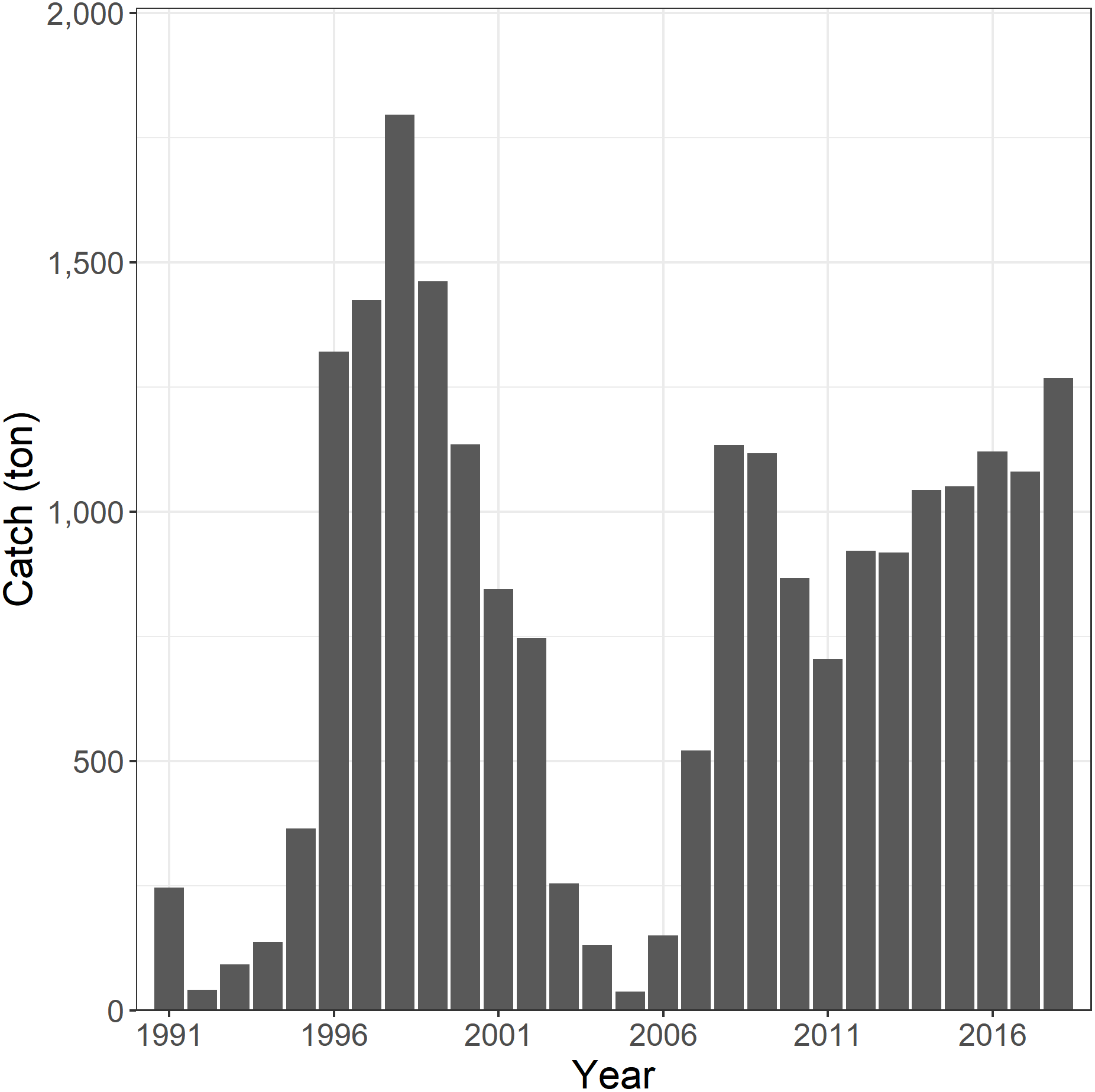
The Korean tuna longline fishery began targeting SBT in the CCSBT convention area in 1991 (Kim et al., 2015). The catch of SBT was initially low but increased to 1,320 tonnes in 1996, peaked at 1,796 tonnes in 1998, and thereafter decreased to below 200 tonnes in the mid-2000s. In 2008, the catch increased again to 1,134 tonnes and thereafter fluctuated in a range of 705–1,268 tonnes due to the national catch limit (Fig. 1).

Figure 1: The annual catch of southern bluefin tuna (SBT) by Korean tuna longline fishery in the CCSBT convention area, 1991–2018.
Trends in CPUE indices are very influential in determining estimates of SBT stock status, and therefore catch quotas. The primary index of abundance used to monitor the adult component of the SBT stock (CCSBT, 2019a) is based on Japanese longline catch and effort data. This index uses a dataset restricted to CCSBT statistical areas 4 to 9 (see Fig. 2 for the area definition), between April and September, and for vessels that have caught a large number of SBT (Itoh, Sakai & Takahashi, 2013; Itoh & Takahashi, 2019). The Japanese dataset comprises much more annual fishing effort and SBT catch, a longer time series, and wider spatial distribution than the Korean dataset. However, as Japanese SBT catches have declined since 1986 (Itoh & Morita, 2021) and, more recently, CPUE has increased (Itoh & Takahashi, 2021), their areas of operation have reduced (Itoh, 2021). Therefore, the need to monitor the indices of other longline fisheries such as Korean and Taiwanese fleets, and the development of joint indices of major longline fleets for the stock assessment has been emphasized.
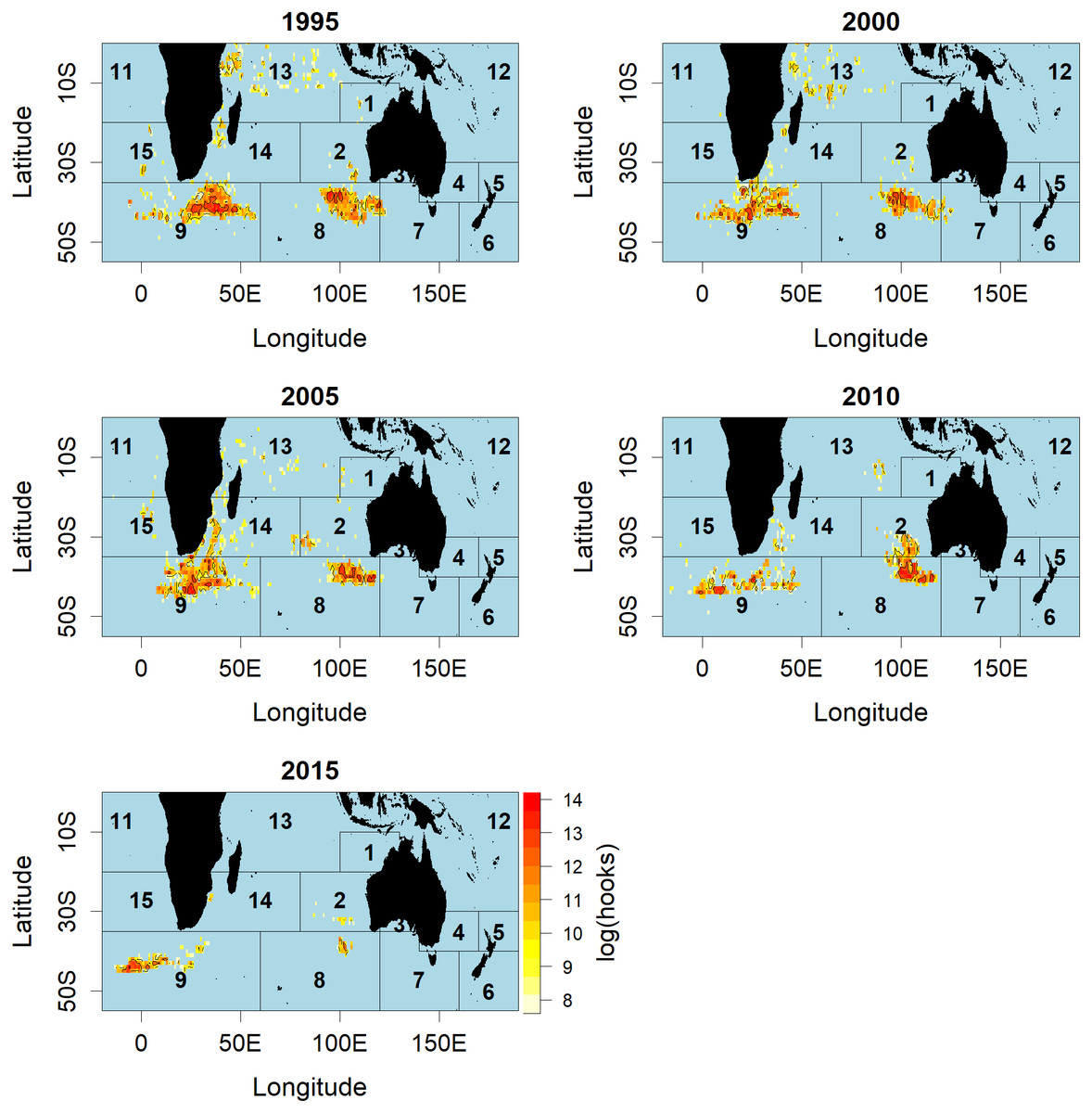
Figure 2: Distributions of fishing effort (hooks) of Korean tuna longline vessels fishing for SBT, aggregated by 5-year period.
Red colour indicates higher fishing effort, and the numbers in the figure indicates the number of CCSBT statistical area used for assessing and managing SBT.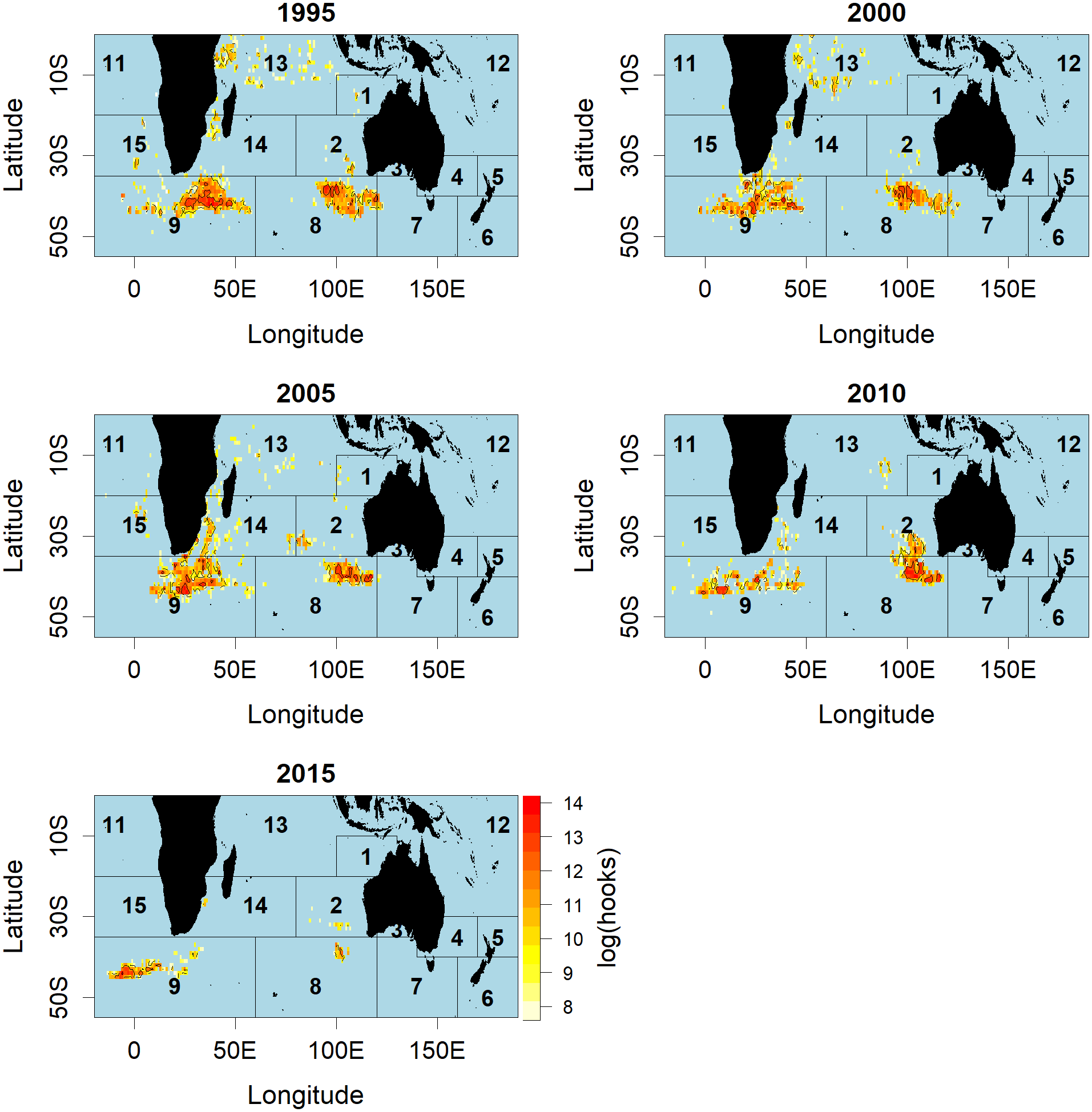
The abundance index described in this paper has been used by the CCSBT as an independent comparison index with the primary index of abundance (CCSBT, 2019a). As well as the independent dataset, this analysis uses different methods for differentiating targeting from the primary CPUE index, in which targeting behaviour is accounted for by including catch rates of bigeye (T. obesus, BET) and yellowfin (T. albacares, YFT) tuna as covariates in the model.
The cluster analysis methods used here are very similar to those used for joint analysis of bigeye, yellowfin, and albacore tuna CPUE in the Indian and Atlantic Oceans (Hoyle et al., 2015; Hoyle et al., 2016; Hoyle et al., 2017; Hoyle et al., 2018; Hoyle et al., 2019a; Hoyle et al., 2019b; Hoyle et al., 2019c; Hoyle et al., 2019d).
In this study, we compare two methods for differentiating targeting practices in the Korean tuna longline data and developing an index of relative abundance. First, we explore the operational set by set data and identify data-based indicators, based on the number of hooks between floats (HBF) and the month, and then use these indicators to subset the data. Secondly, we use cluster analysis to group the effort into fishing strategies based on the species composition of the catch. Then, SBT CPUE is standardized using two methods based on the lognormal constant model and the delta lognormal approach.
Data & Methods
Data
Set by set catch and effort data were compiled by the Korean National Institute of Fisheries Science (NIFS). Data were selected with the criterion that when a vessel reported the capture of at least one SBT in a month, all effort for the vessel-month was included.
The fields reported in the operational set by set data were vessel identifier (call sign), fishing location to 1° cell of latitude and longitude, date, effort (number of hooks and floats), and catch in numbers of southern bluefin tuna (SBT), bigeye (BET), yellowfin (YFT), albacore (ALB), skipjack (SKJ), swordfish (SWO), black marlin (BLM), blue marlin (BUM), striped marlin (MLS), sailfish (SFA), sharks (SHA), and other species (OTH).
Data used in this study were from 1996 to 2018. Data prior to 1996 were not available due to insufficient information for CPUE standardization. Dates were converted to months and quarters. Since Korean longliners set at night or at dawn, moon phase was used to calculate the relative lunar illumination for each date, using the R package lunar (Lazaridis, 2014). Spatial positions were classified into 5° cells, and CCSBT statistical areas (CCSBT, 2019b). The numbers of hooks between floats (HBF) were calculated by dividing hooks by floats and rounding to the nearest whole number.
For CPUE standardization, data were cleaned by removing sets in which there were fewer than 1,000 hooks or more than 5,000 hooks. Korean tuna longline vessels fishing for SBT in the CCSBT convention area have individual annual quotas. The fishing season is from April to March of the following year. They have mainly operated in two locations to the south of 35°S, either between 10°W and 50°E (within CCSBT statistical area 9) or between 90°E and 120°E (within CCSBT statistical area 8) (Fig. 2). Effort has focused on the western area (statistical area 9) from March to September/October and shifted to the eastern area (statistical area 8) from July/August until December (Fig. 3). For that reason, we defined two separate core SBT fishing areas: within statistical area 9 from March to October and statistical area 8 from July to December.
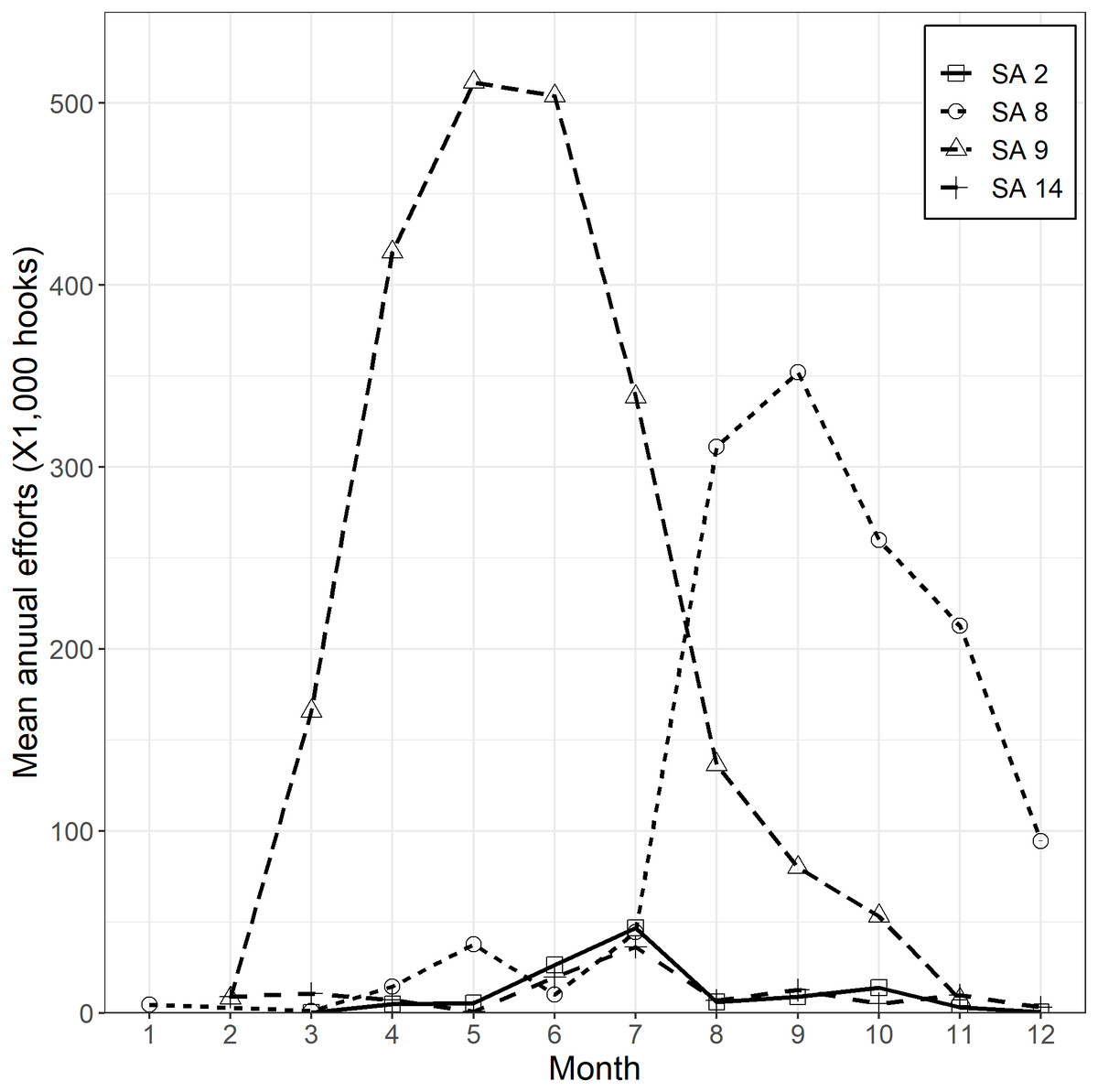
Figure 3: Mean annual fishing efforts (hooks) by month and CCSBT statistical area (SA).
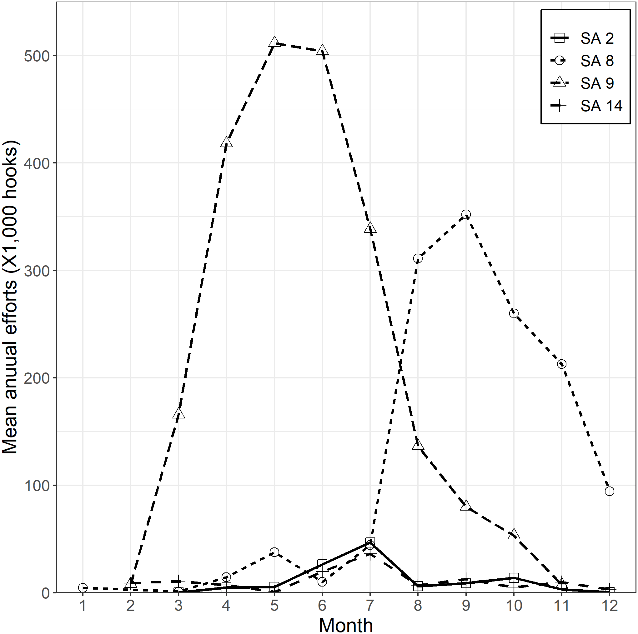
Data exploration
Data were plotted to explore the spatial and temporal distributions of effort, and patterns in operational characteristics such as the hooks per set and HBF. Operational characteristics were compared with catch rates to identify possible gear-based criteria for targeting. We examined patterns through time and among major species in the nominal catch rates by year-quarter and area and compared them with patterns in the proportions of sets with no catch of each species. We plotted maps of the species composition through time, to identify possible spatial and temporal variation in fishing behaviour or population composition.
To further explore changes in the fishery and identify periods of change, we plotted the participation of vessels in the fleet, sorted first by the start date and then by the end date of participation in the fishery. To explore changes in effort distribution and concentration through time, we plotted the numbers of 5° × 5° and 1° × 1° cells fished and the average number of operations per fished cell for each year and area.
Target change
Target change can be a significant problem for CPUE standardization since it can bias CPUE trends. Analyses were carried out using two alternative approaches to differentiate targeting practices.
Data selection
Gear depth and gear configuration are considered important factors in CPUE standardization, and HBF has often been used as an indicator of fishing depth and target species for tuna longliners (e.g., Okamoto, Yokawa & Chang, 2005). Therefore, based on results of the data exploration analysis, we included only effort that met gear criteria based on HBF, and was within the core periods of SBT targeting in each area. This approach removed effort considered unlikely to have targeted SBT and allowed the analysis to focus on effort targeting SBT.
Cluster analysis
Species compositions were analysed to identify groups potentially using different targeting strategies, and cluster IDs used as categorical variables in the standardization model.
All data for the statistical areas 8 and 9 were clustered following Hoyle et al. (2015). Sets with no catch of any species were removed, and remaining data aggregated by vessel-month. Species composition varies among sets due to the randomness of chance encounters between fishing gear and schools of fish, which can lead clustering to misallocate some sets. Aggregating the data reduces this variability and the rate of misallocation, if individual vessels follow a consistent fishing strategy through time. However, misallocation can occur when vessels change their fishing strategy within the aggregation period. We aggregated the data by vessel-month, based on the understanding that the Korean fleet mostly operate with consistent strategies over a long period.
We calculated proportional species composition by dividing the catch-in-numbers of each species by catch-in-numbers of all species in the vessel-month. Thus, the species composition values of each vessel-month summed to 1, ensuring that large and small catches were given equivalent weight. The data were transformed by centring and scaling, to reduce the dominance of species with higher average catches. Centring was performed by subtracting the column (species) mean from each column, and scaling was performed by dividing the centred columns by their standard deviations.
Data were clustered using the hierarchical Ward hclust method, implemented with function hclust in R, option ‘Ward.D’, after generating a Euclidean dissimilarity structure with function dist. This approach differs from the standard Ward D method which can be implemented by either taking the square of the dissimilarity matrix or using method ‘ward.D2’ (Murtagh & Legendre, 2014). However in practice the method gives patterns of clusters that are more consistent with expert understanding of fishing behaviour than ‘ward.D2’ (Hoyle et al., 2015).
Data were also clustered using the kmeans method, which minimizes the sum of squares from points to the cluster centres, using the algorithm of Hartigan & Wong (1979). It was implemented using function kmeans in the R stats package (R Core Team, 2016).
Approaches used to select the appropriate number of clusters suggested similar numbers of groups. First, we considered the number of major targeting strategies likely to appear in the dataset, based on understanding and exploration of the data. Second, we applied hclust to transformed vessel-month level data and examined the hierarchical trees, subjectively estimating the number of distinct branches. Third, we ran kmeans analyses on untransformed vessel-month level data with number of groups k ranging from 2 to 25, and plotted the deviance against k. The optimal group number was the lowest value of k after which the rate of decline of deviance became slower and smoother. Finally, following Winker, Kerwath & Attwood (2014) we applied the nScree function from the R nFactors package (Raiche & Magis, 2010), which uses various approaches (Scree test, Kaiser rule, parallel analysis, optimal coordinates, acceleration factor) to estimate the number of components to retain in an exploratory principal component analysis (PCA).
We plotted the hclust clusters to explore the relationships between them and the species composition and other variables, such as HBF, number of hooks, year, and fishing location. Plots include beanplots of the distributions of variables by cluster and the proportion of each species in the catch by cluster, and maps of the spatial distribution for each cluster.
GLM analyses
SBT CPUE was standardized using the set by set data and generalized linear models (GLMs) in Microsoft R Open 3.3.2 (R Core Team, 2016), and the methods generally followed the approaches used by Hoyle & Okamoto (2011) and Hoyle et al. (2015). Analyses were conducted separately for each of the two core areas, and for each of the two target change methods.
Data were prepared by selecting data for vessels that had made at least 100 sets, for years in which there had been at least 100 sets, and for 5° cells in which there had been at least 200 sets. Categories with too few sets provide estimates with high uncertainty and low reliability, so this approach removes a few cells, vessels, and time periods that lack much usable information.
The CPUE standardization was carried out using generalized linear models (GLMs) with both a lognormal constant model and a delta lognormal approach. The lognormal constant GLM was used to summarize the effects of covariates on the index (via the package influ, Bentley et al., 2011) across the whole dataset, but was not used for inferences about the abundance trend, since this approach has been superseded by methods that model zeroes more directly (Maunder & Punt, 2004). The preferred abundance indices were obtained using the delta lognormal approach.
Covariates for all models were specified as . The functions λ, g and h were cubic splines with 5, 3, and 4 degrees of freedom, respectively, with sufficient flexibility to explain variability while avoiding overfitting. Higher order terms are inadvisable for conventional polynomials but perform relatively well with regression splines (Harrell, 2001). The number of hooks (hooks) was included in the model to allow for possible hook saturation and potential targeting changes associated with hooks per set. The variable moon was the lunar illumination on the date of the set, which was included to find out whether SBT catch rate is related to moon phase. The variables year, vessid, and latlong (5° latitude-longitude cell) were fitted as categorical variables. For the clustering-based approach, the cluster was also included as a categorical variable.
The models did not include HBF directly. The data selection method had already addressed HBF by including only a narrow range of HBF values in the range 9–12. The cluster analysis method addresses targeting independently of HBF, and in any case, less than 1% of sets included HBF outside the 9–12 range.
The following lognormal model was used.
The units of the input CPUE is catch-in-number of SBT per 100 hooks, and the constant k, added to allow for modelling sets with zero catches of the species of interest, is 10% of the mean CPUE for all sets (Campbell, 2004).
The delta lognormal approach (Lo, Jacobson & Squire, 1992; Maunder & Punt, 2004) used a binomial distribution for the probability w of catch rate being zero and a probability distribution f (y), where y was log (catch/hooks per set), for non-zero (positive) catch rates.
where g is the logistic function.
Data in the models were ‘area-weighted’, with the statistical weights of the sets adjusted so that the total weight per year in each 5° cell would sum to 1. This method was based on the approach identified using simulation by Punsly (1987) and Campbell (2004), that for set j in area i and year t with hooks hijt, the weighting function that gave the least average bias was: . Given the relatively low variation in number of hooks between sets in a stratum, we simplified this to .
The models had no interactions between year effects and other covariates, so relative annual expected responses for the lognormal constant index and the lognormal component of the delta lognormal index were invariant with different values of other covariates. We generated an index for each of these models by predicting the response for each year with covariate values held constant.
For the delta model, however, the annual trend is affected by the values chosen for the other covariates, which are held constant when predicting annual catch rates. Choosing covariate values that give a higher rate of nonzero catch will reduce the variability among years in the delta index, and hence in combined index. To avoid subjectivity, the constant used to predict from the delta regression was adjusted so that the mean of the annual proportions of positive catches was the same in the predictions as in the observed data.
The combined index estimated for each year was the product of the year effects for the two model components, . This index was normalized to average 1, so the final index represents relative catch rate.
Model fits were examined by plotting the residual densities and using Q–Q plots.
Results
Data exploration
Almost all Korean tuna longline vessels fishing for SBT used between 9 and 12 HBF (Fig. 4), with the majority of HBF outside this range coming from north of 35°S, outside the main SBT targeting area. The number of hooks per set has been relatively consistent since 1996, averaging a little over 3,000.
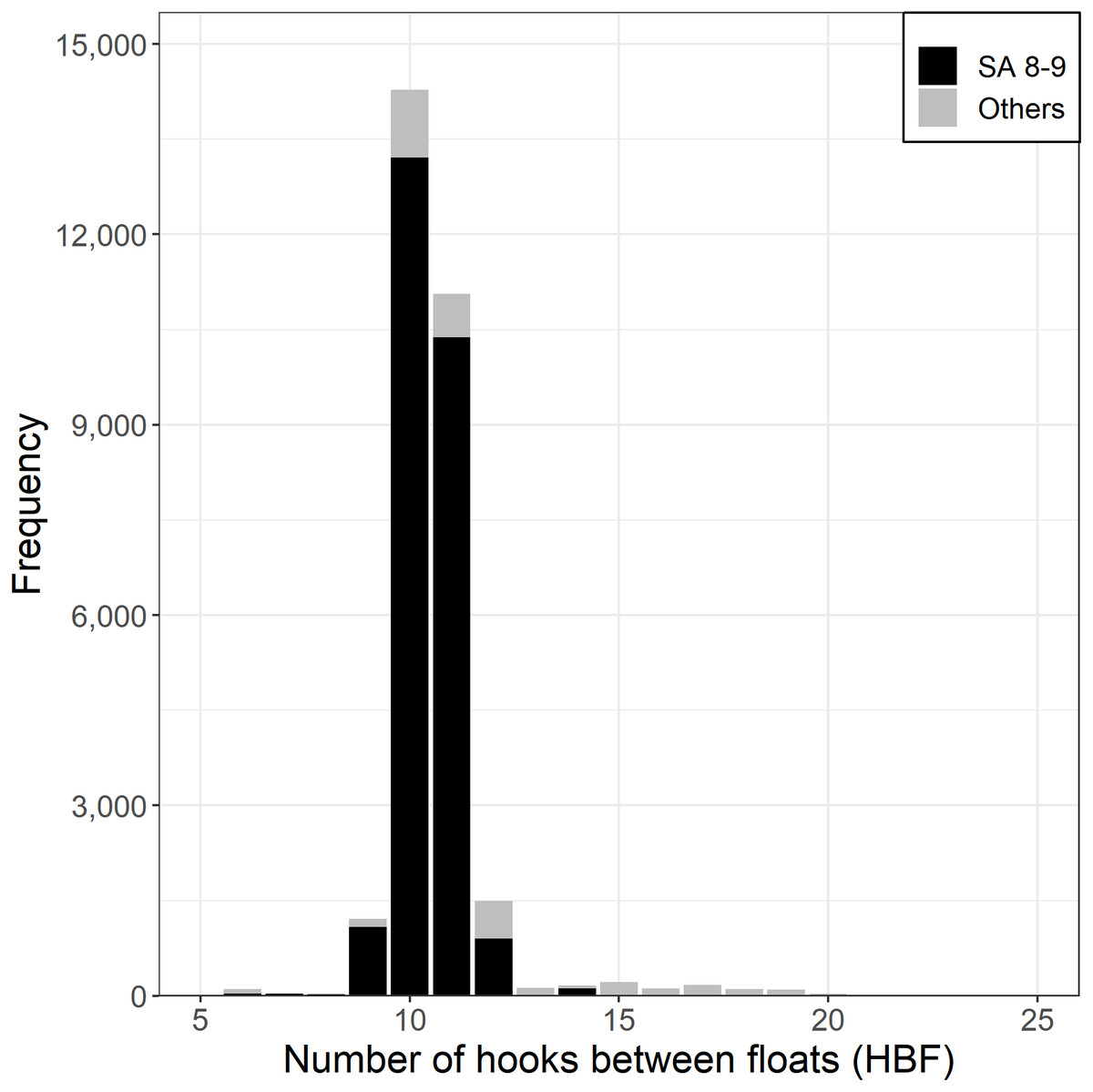
Figure 4: Frequency of hooks between floats (HBF) for the main fishing ground with the darker shade for CCSBT statistical areas (SA) 8 and 9, and the lighter shade for other areas.
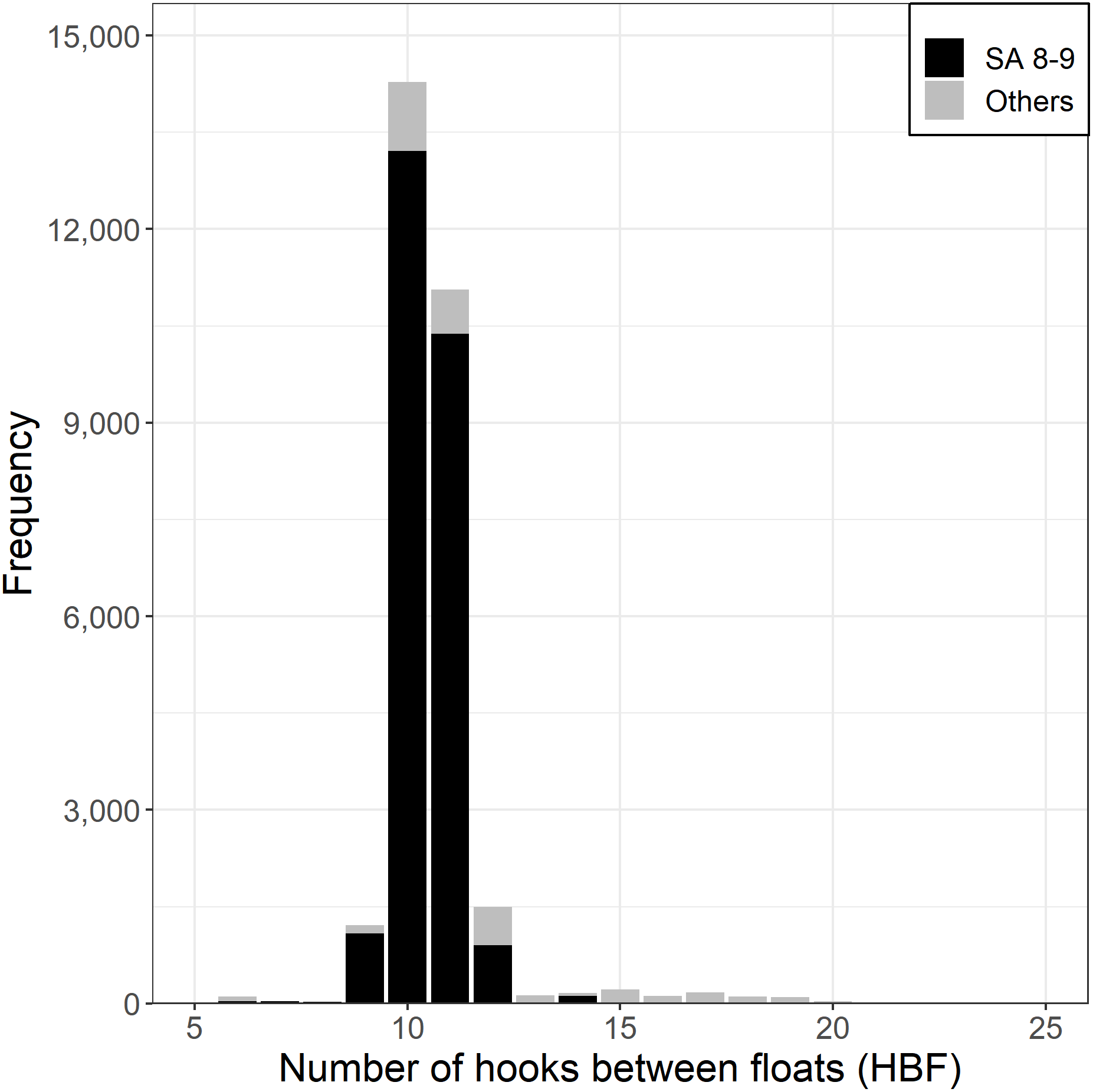
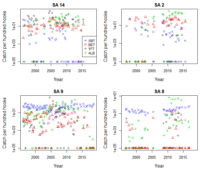
Mean nominal catch rates in statistical areas 8 and 9 were higher for SBT than for other species until the mid-2000s (Fig. S1). After this time in the areas 8 and 9 the SBT catch rates decreased and other species, particularly albacore tuna (ALB), increased. However, in the most recent years the SBT catch rates were again higher than other species. Similarly, the proportion of sets reported with zero SBT catches was low through most of the time series in the areas 8 and 9, but increased from 2004 to 2010 in area 9 and in some years during the early 2010s in area 8 (Fig. S2).
Statistical areas 2 and 14 in the Indian Ocean are at temperate latitudes between 20°S and 35°S. Highest catch rates were for YFT and more recently ALB in area 14, and BET and ALB in area 2 (Fig. S1). Since the mid-2000s ALB catch rates have increased markedly and particularly in the area 2, suggesting a trend towards targeting this species. Catch rates of SBT have been relatively low throughout the period, consistent with a high proportion of zero catches of SBT (Fig. S2), suggesting little or no targeting of SBT by Korean tuna longline vessels in these areas.
Figure 5 shows spatial patterns of SBT and ALB as proportions of the total reported catch south of 30°S by 5-year period. The SBT proportion was high in all periods, increasing further south, but declined in all areas after 2005. In the 2010s, particularly, there was little SBT taken in statistical area 8 north of about 37°S, whereas a high proportion of the catch in this area was ALB. This appears to reflect spatially and temporally differentiated targeting in area 8.
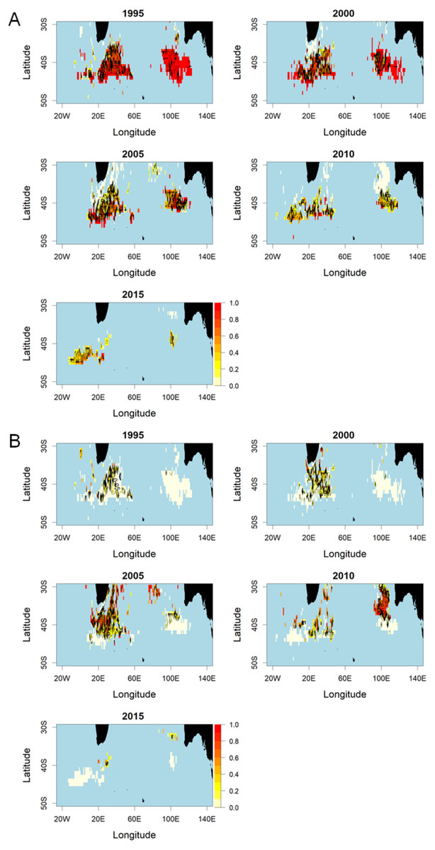
Figure 5: Proportions of SBT and ALB in the total catch in numbers by 1° cell, aggregated over 5 years within the period 1996–2018.
Red colour indicates a higher proportion of the catch. (A) Southern bluefin tuna (SBT). (B) Albacore tuna (ALB).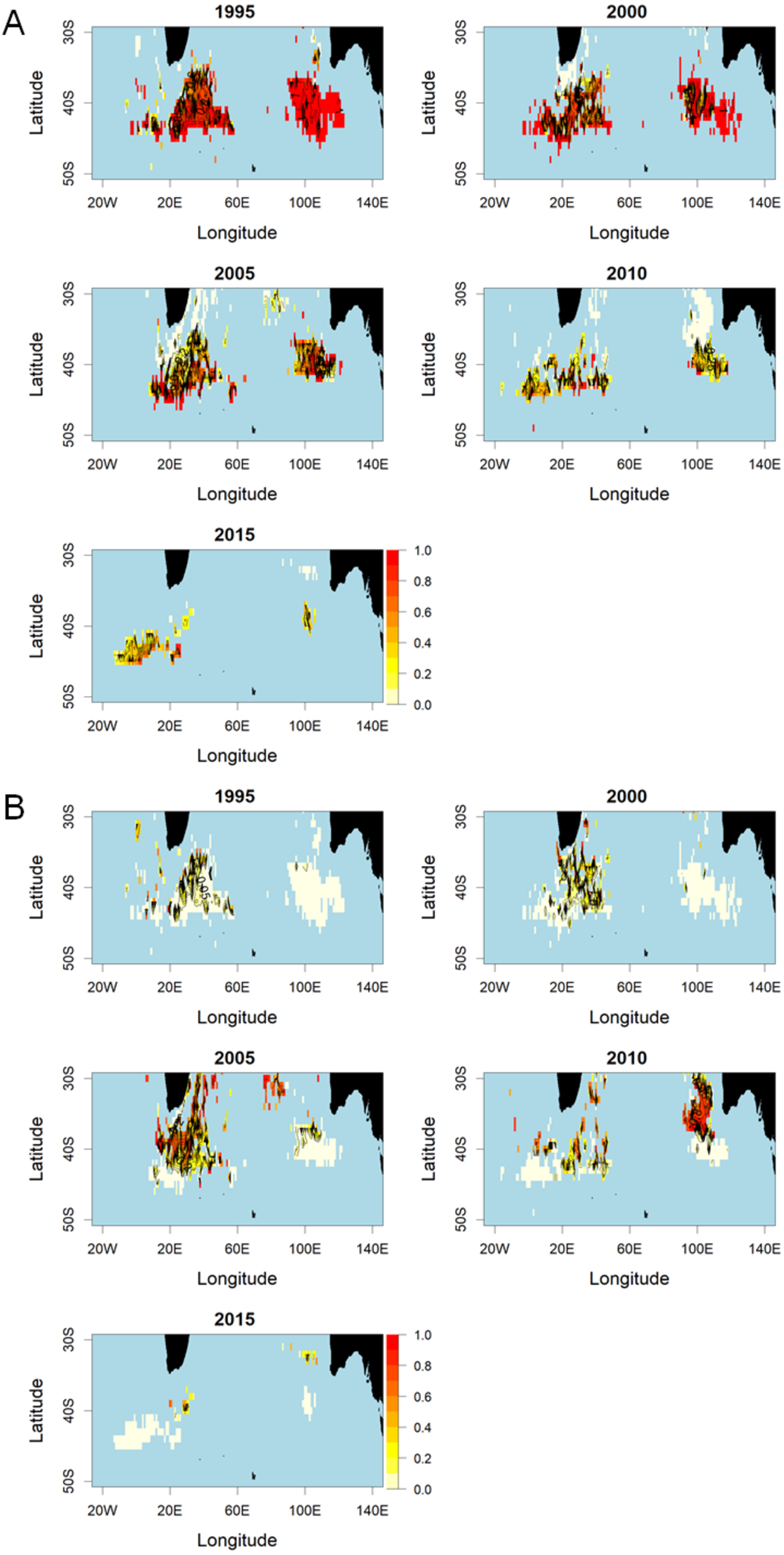
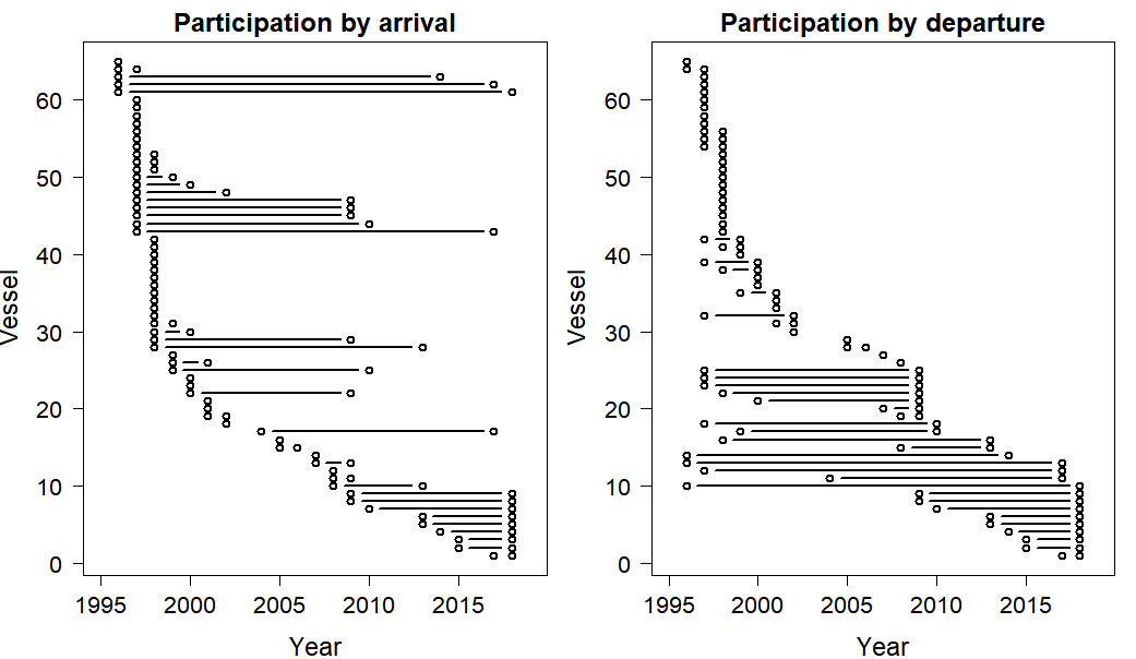
Sixty-five Korean tuna longline vessels have participated in statistical areas 8 and 9 since 1996 (Fig. S3), with over half of the fleet reporting their first participation before 2000. New vessels have arrived slowly but regularly. Vessel turnover was initially high, with over 20 vessels having stopped participating by 1998. In 2010, many vessels stopped participating because the SBT stock was at a critical stage, about 5% or less of the unfished spawning biomass level, and the quota was greatly reduced (CCSBT, 2009a; CCSBT, 2009b), and since then eight more have stopped but seven others have joined the fishery.
The total number of major cells (5° × 5° × month) fished has varied annually but declined considerably since the peak in 2009 (Fig. 6A). Over the same period, effort has become more concentrated with more operations per cell. This increasing concentration is also apparent at the minor cell (1° × 1° × month) level (Fig. 6B). The distribution of effort within major cells was more stable until recently, with similar numbers of minor cells per major cell on average, but in 2017-2018 increased to the highest level yet seen (Fig. 6C). Since 2008 the timing of effort in statistical areas 8 and 9 has changed, gradually moving earlier in the year, though with different timing peaks in each area.
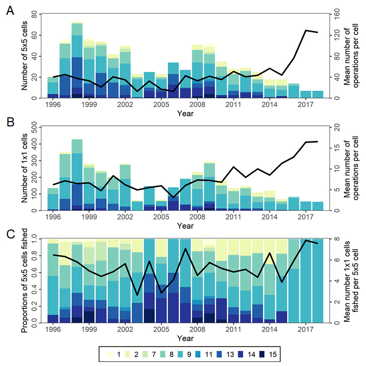
Figure 6: The number of cells fished and the mean annual number of longline operations per cell in CCSBT statistical areas, 1996–2018.
(A) Bar and the line represent the number of major cells (5° × 5° by month) fished by CCSBT statistical area and year, and the mean annual operations per cell, respectively. (B) Bar and the line represent the number of minor cells (1° × 1° by month) fished by CCSBT statistical area and year, and the mean annual operations per cell, respectively. (C) Bar and the line represent relative distribution of fished major cells as the proportion of the cell fished by CCSBT statistical area, and the mean number of minor cells fished per major cell by year, respectively.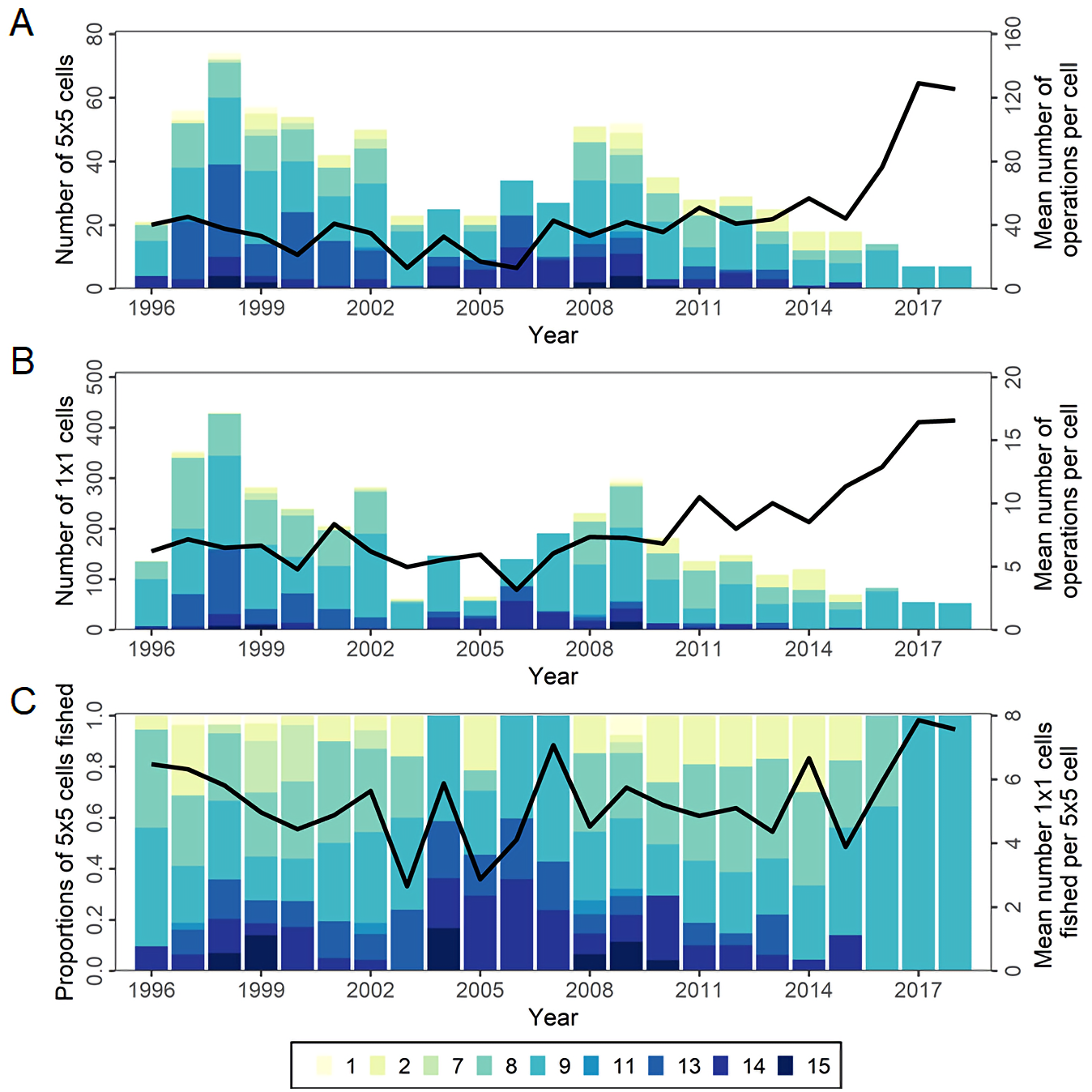
Target change
Data selection
Based on data exploration, the data selection method firstly removed sets in which HBF was less than 9 or greater than 12 that were mainly used in the non-main SBT fishing grounds (Fig. 4). Secondly, data for each area were selected for the periods in which most SBT were caught (Fig. S4), so as to avoid periods when other species were targeted. Data for statistical area 8 were included for the months July to December, and data for statistical area 9 were included for March to October (Fig. 3).
Clustering
Applying Ward’s D hierarchical cluster analysis at the vessel-month level identified strong separation among two to three groups in statistical areas 8 and 9 (Fig. 7), so three clusters were chosen in each area to consider major targeting strategies. We preferred to use more clusters where there was uncertainty because unresolved target change can cause bias in indices.
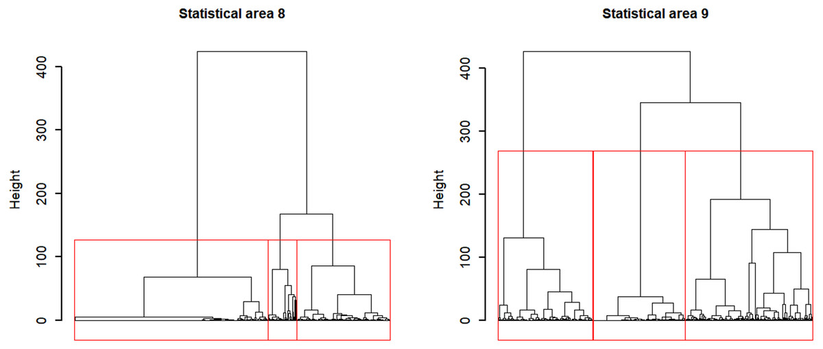
Figure 7: Dendrograms for Ward hierarchical cluster analyses of CCSBT statistical areas 8 and 9, with the red lines indicating the separation into three clusters for each.
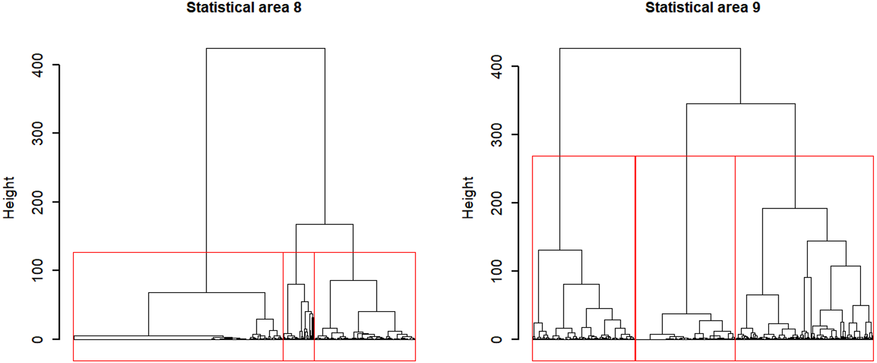
In statistical area 8 (Figs. 8, 9 and 10), the species composition of cluster 2 was dominated by SBT, with small amounts of other species groups. Cluster 3 included similar amount of SBT, SHA and OTH, while cluster 1 included more ALB than SBT, with some OTH, YFT and BET. The SBT cluster 2 dominated the early part of the time series, with clusters 1 and 3 more apparent after 2005. Cluster 1 was represented during March to June, while clusters 2 and 3 occurred mostly in the second half of the year. Cluster 2 was fewer HBF than the average, while the hooks per set were similar for all clusters. Cluster 2 was well represented across most of the fished area, while cluster 3 occurred at middle latitudes from about 38°S–42°S, and cluster 1 occurred almost entirely in the far north of the area.
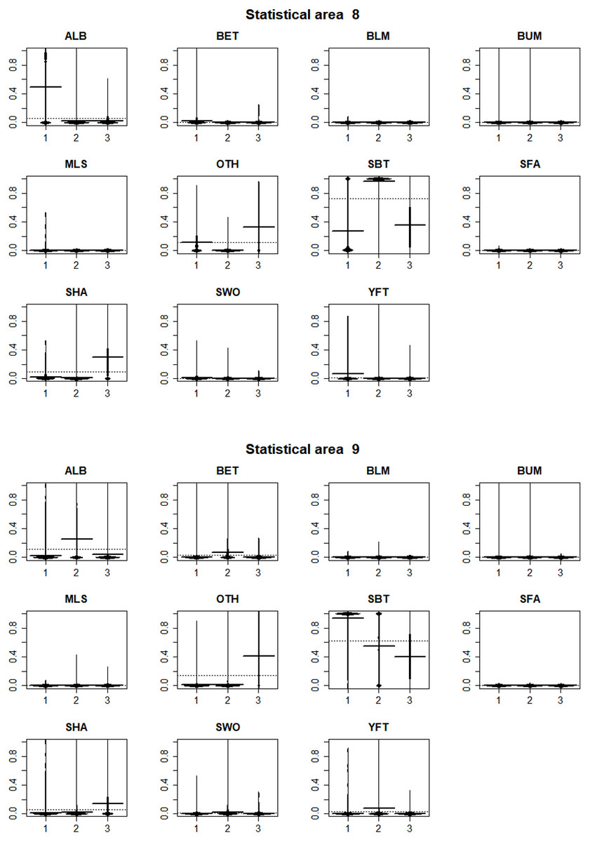
Figure 8: Beanplots showing species composition by cluster for statistical areas 8 and 9.
The horizontal bars indicate the medians.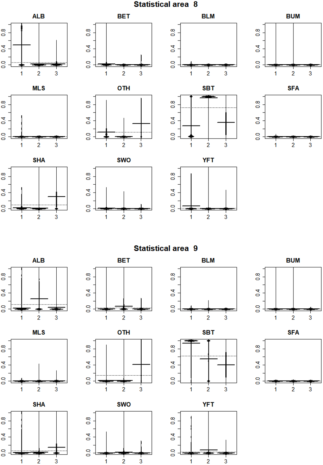
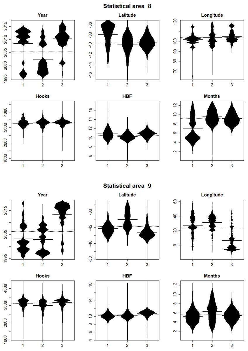
Figure 9: Beanplots showing the distributions of sets versus covariate by cluster for CCSBT statistical areas 8 and 9.
The horizontal bars indicate the medians.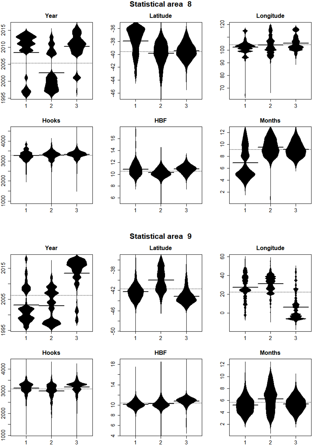
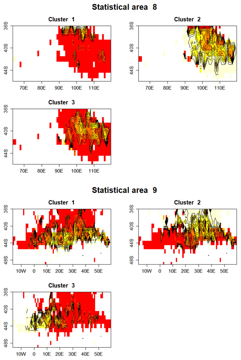
Figure 10: Maps showing the proportion of each cluster per 1 degree cell in total effort for CCSBT statistical areas 8 and 9.
Higher proportions are shown in yellow, and white space indicates no reported effort.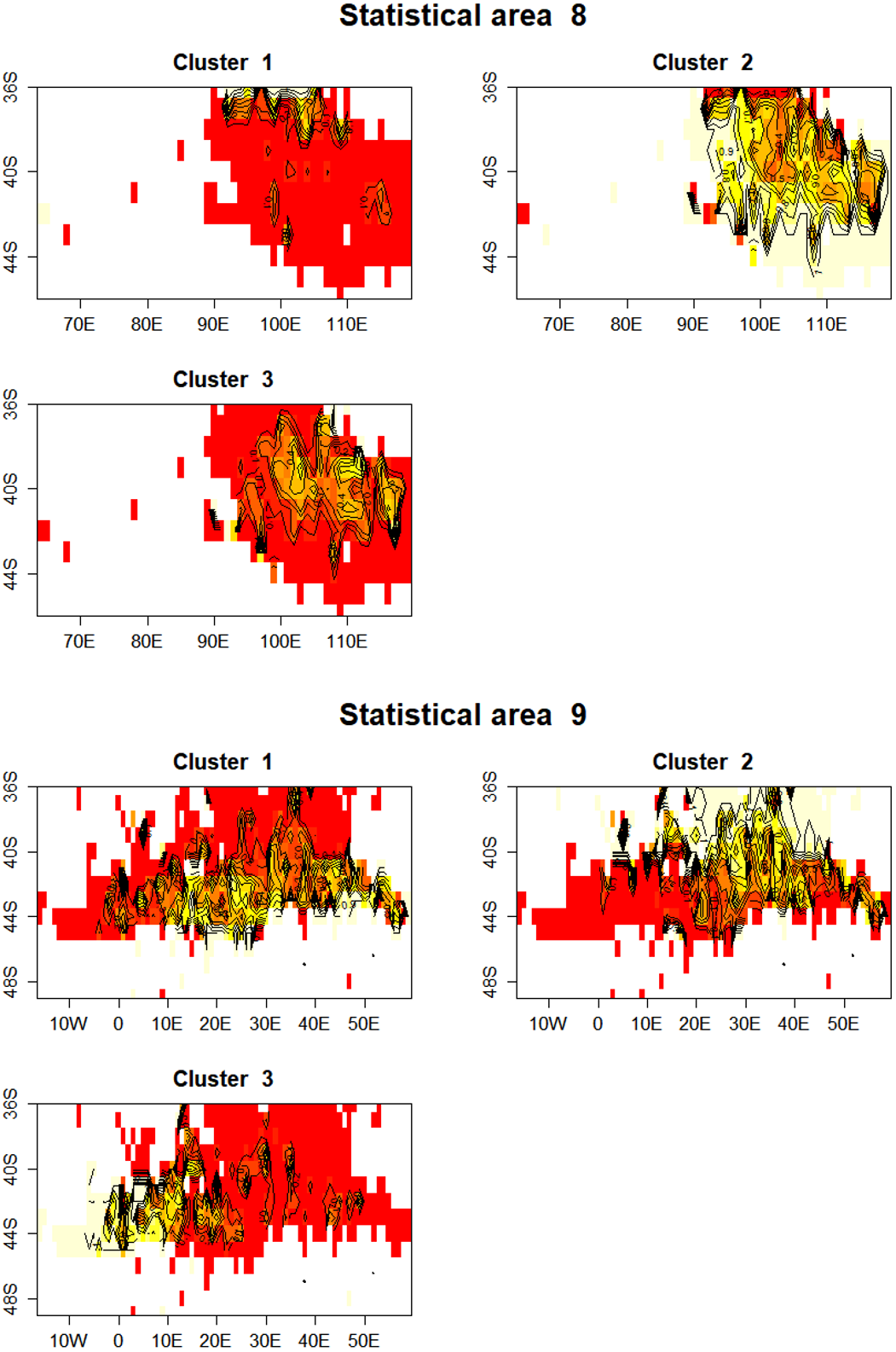
In statistical area 9 (Figs. 8–10), cluster 1 comprised almost entirely SBT, with small amounts of ALB and BET. Cluster 2 included significant SBT along with ALB, and some BET and YFT. Cluster 3 included similar amounts of SBT and OTH, with some SHA and ALB. Clusters 1, 2, and 3 were more strongly represented in the early, middle, and later parts of the time series, respectively. Clusters 1 and 3 occurred mostly in the period before August, while cluster 2 extended into October. The mean number of hooks was higher in cluster 3 and lower in cluster 2, and cluster 3 also had slightly more HBF. Cluster 2 dominated the northeast of area 9, while clusters 1 and 3 dominated the southeast and the southwest, respectively.
In summary, results show that effort in clusters 1 and 2 targeted ALB in area 8 and area 9, respectively. ALB targeting clusters operated further north than those targeting SBT. The main fishing periods for the ALB clusters were before June in area 8 and after June in area 9, whereas SBT targeting occurred after and before June, respectively.
CPUE standardization
All explanatory variables in the lognormal constant models and the lognormal components of the delta lognormal were statistically significant based on AIC (Table 1), with the year, location (latlong), vessel (vessid), and month effects the most important. The cluster effect was also important in statistical area 8, but less so in area 9. Several variables in the binomial component with weak support were retained in the model for consistency with the lognormal component, and because they had little effect on the results given the high rates of nonzero catches.
| (A) | ||||||||||||
|---|---|---|---|---|---|---|---|---|---|---|---|---|
| Variable | Data selection | Clustering analysis | ||||||||||
| Statistical area 8 | Statistical area 9 | Statistical area 8 | Statistical area 9 | |||||||||
| df | dev | ΔAIC | df | dev | ΔAIC | df | dev | ΔAIC | df | dev | ΔAIC | |
| <none > | 35.6 | 0 | 148.4 | 0 | 43.3 | 0 | 147.8 | 0 | ||||
| Year | 14 | 42.0 | 1,397 | 22 | 177.1 | 2,742 | 14 | 47.7 | 873 | 22 | 171.1 | 2,310 |
| Latlong | 10 | 37.0 | 298 | 18 | 160.1 | 1,162 | 10 | 44.7 | 274 | 18 | 159.1 | 1,145 |
| Hooks | 5 | 35.8 | 41 | 5 | 150.4 | 198 | 5 | 43.4 | 16 | 5 | 149.3 | 157 |
| Vessid | 26 | 37.4 | 361 | 35 | 159.0 | 1,011 | 26 | 46.2 | 549 | 35 | 158.0 | 1,009 |
| Month | 3 | 36.8 | 265 | 3 | 156.9 | 869 | 3 | 44.5 | 239 | 3 | 156.3 | 900 |
| Moon | 4 | 36.5 | 192 | 4 | 148.6 | 10 | 4 | 44.1 | 158 | 4 | 147.9 | 9 |
| Cluster | – | – | – | – | – | – | 2 | 45.7 | 505 | 2 | 148.7 | 100 |
| (B) | ||||||||||||||||||||
|---|---|---|---|---|---|---|---|---|---|---|---|---|---|---|---|---|---|---|---|---|
| Variable | Data selection | Clustering analysis | ||||||||||||||||||
| Statistical area 8 | Statistical area 9 | Statistical area 8 | Statistical area 9 | |||||||||||||||||
| Binomial probability | Lognormal positive | Binomial probability | Lognormal positive | Binomial probability | Lognormal positive | Binomial probability | Lognormal positive | |||||||||||||
| df | dev | ΔAIC | dev | ΔAIC | df | dev | ΔAIC | dev | ΔAIC | df | dev | ΔAIC | dev | ΔAIC | df | dev | ΔAIC | dev | ΔAIC | |
| <none > | 328.9 | 0 | 50.0 | 0 | 2194.2 | 0 | 164.8 | 0 | 788.7 | 0 | 55.6 | 0 | 2222.0 | 0 | 165.0 | 0 | ||||
| Year | 14 | 354.3 | −3 | 58.6 | 1,348 | 22 | 2548.9 | 311 | 197.0 | 2,623 | 14 | 865.2 | 49 | 61.8 | 930 | 22 | 2500.7 | 235 | 190.3 | 2,134 |
| Latlong | 10 | 355.7 | 7 | 51.7 | 276 | 18 | 3048.7 | 818 | 182.3 | 1,470 | 10 | 821.8 | 13 | 57.3 | 253 | 18 | 3000.7 | 743 | 182.7 | 1,524 |
| Hooks | 5 | 342.1 | 3 | 50.2 | 32 | 5 | 2270.1 | 66 | 166.0 | 99 | 5 | 807.6 | 9 | 55.7 | 9 | 5 | 2297.8 | 66 | 160.0 | 83 |
| Vessid | 26 | 356.9 | −24 | 52.5 | 369 | 35 | 2349.5 | 85 | 172.5 | 607 | 26 | 838.1 | −3 | 59.0 | 494 | 35 | 2364.3 | 72 | 172.9 | 644 |
| Month | 3 | 336.9 | 2 | 51.5 | 241 | 3 | 2327.3 | 127 | 169.1 | 375 | 3 | 793.7 | −1 | 57.1 | 234 | 3 | 2351.8 | 124 | 169.3 | 393 |
| Moon | 4 | 333.7 | −3 | 51.2 | 200 | 4 | 2196.2 | −6 | 166.1 | 102 | 4 | 793.2 | −3 | 56.8 | 187 | 4 | 2223.5 | −7 | 166.3 | 116 |
| Cluster | – | – | – | – | – | – | – | – | – | – | 2 | 874.1 | 81 | 57.3 | 274 | 2 | 2239.5 | 13 | 166.0 | 91 |
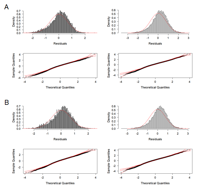
Nominal and standardized CPUE indices were developed for SBT in statistical areas 8 and 9, based on lognormal constant and delta lognormal models using data selection and cluster analysis (Fig. 11). The two methods to address targeting led to very similar standardized indices, with small differences from the nominal CPUE trend. Diagnostic frequency distributions and QQ-plots suggest that the data fitted the GLMs adequately (Figs. S5 and S6).
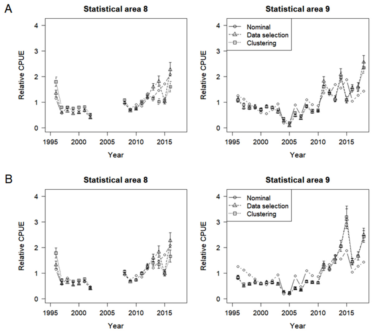
Figure 11: Nominal and standardized CPUE indices based on lognormal constant models and delta lognormal models for CCSBT statistical areas 8 and 9, addressing target change using selected data and cluster analysis.
(A) Lognormal constant models. (B) Delta lognormal models.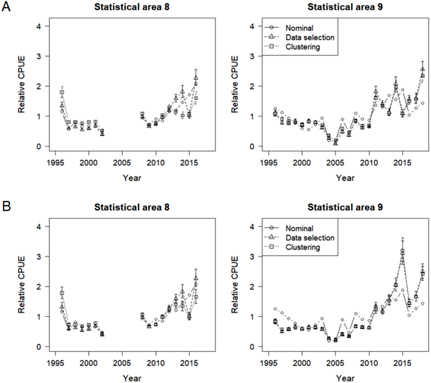
Differences between the targeting analysis methods were similar for both the lognormal constant and delta lognormal indices, though slightly larger for the lognormal constant method. The main differences between the methods occurred in the late 2000s for area 9 and in the 2013-2014 period for area 8, when indices were lower for the clustered data than the selected data. This may be because delta lognormal models are better than lognormal constant models at dealing with zero catches.
In addition, the area 9 delta lognormal indices differed from the lognormal constant indices. They were markedly lower before 2005 and were considerably higher in 2015 and 2018 but had similar trends to the nominal CPUEs in the recent years.
Hence the indices provided by the delta lognormal indices using the clustered data were chosen as the representative indices for SBT caught by the Korean tuna longline fishery. In summary, patterns in the indices differ somewhat between the statistical area 8 and 9 (Fig. 11B). Both sets of indices decreased until the mid-2000s, and subsequently increased, particularly in the last few years. However, lack of data prevents estimation for area 8 in the periods 2003-2007 and since 2017. Recent effort in area 8 is too low and concentrated to provide reliable estimates.
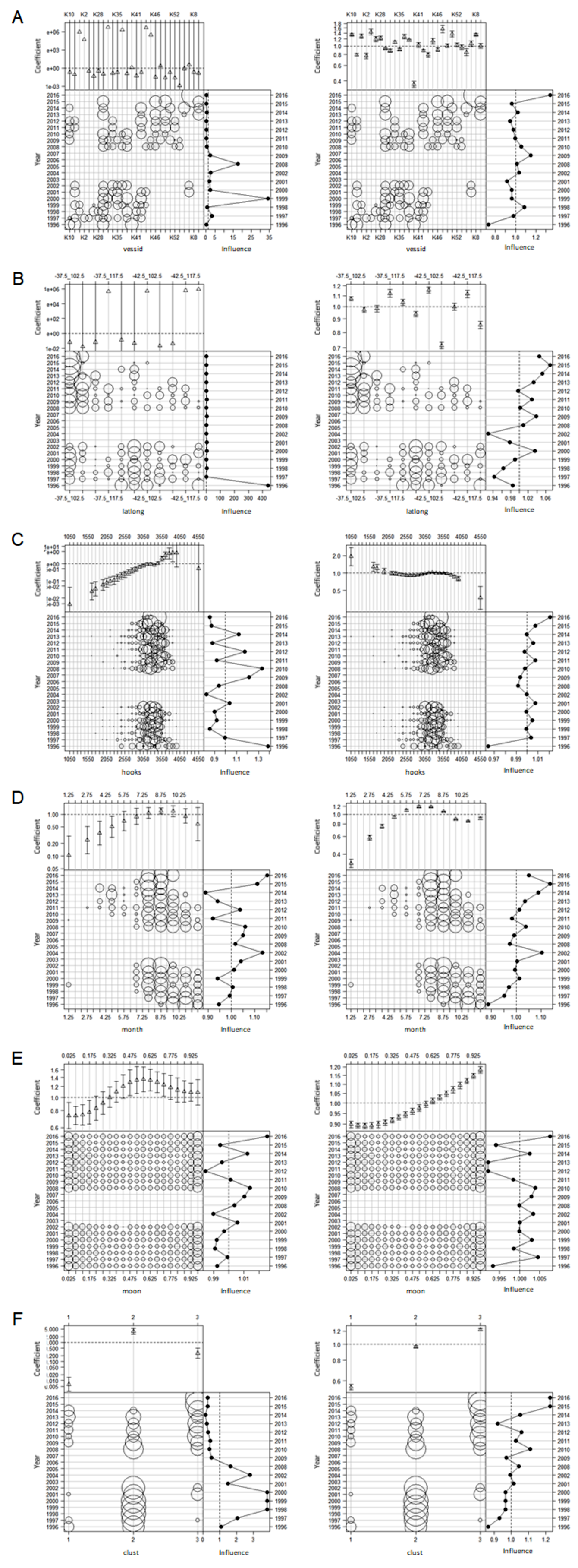
Influence plots for each covariate in the lognormal constant model using the clustered data are presented in Fig. 12, and those for the binomial and lognormal positive components in the delta lognormal model are presented in Figs. S7 and S8. Each subplot has three components, with the parameter estimates for each covariate level at the top, the effort by time interval and covariate level indicated by circle areas in the lower left component, and the cumulative influence of the covariate on the year effect on the right. Each subplot reports influence on a different scale, so the scales must be considered when comparing the relative importance of each covariate.
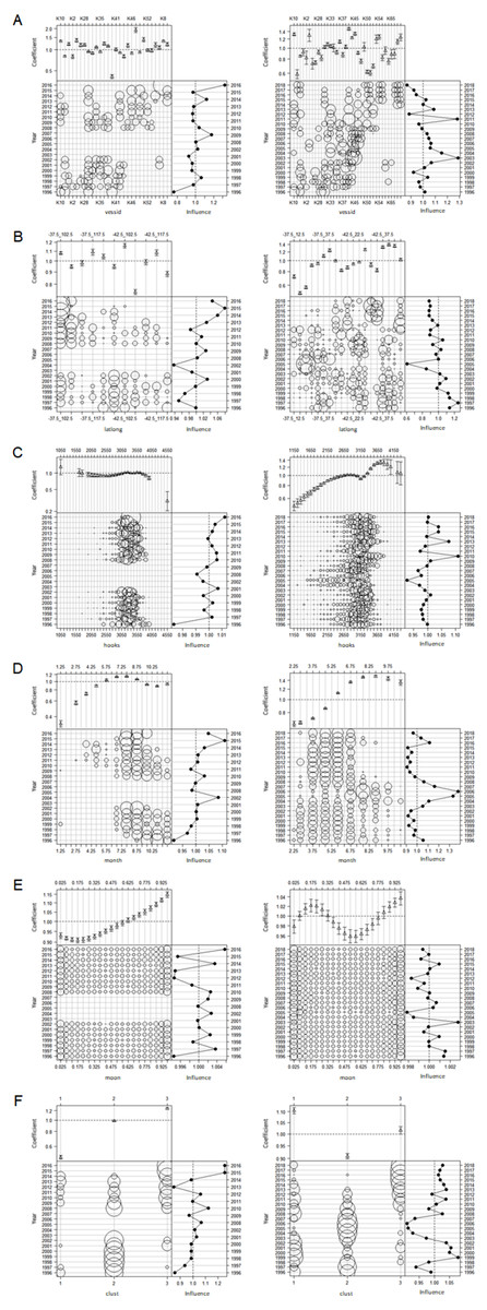
Figure 12: Influence plots for each effect for lognormal constant model of CCSBT statistical areas 8 (left) and 9 (right), addressing target change using clustering.
(A) Vessel effects. (B) Spatial (lat-long) effects. (C) Hooks effects. (D) Month effects. (E) Moon effects. (F) Cluster effects.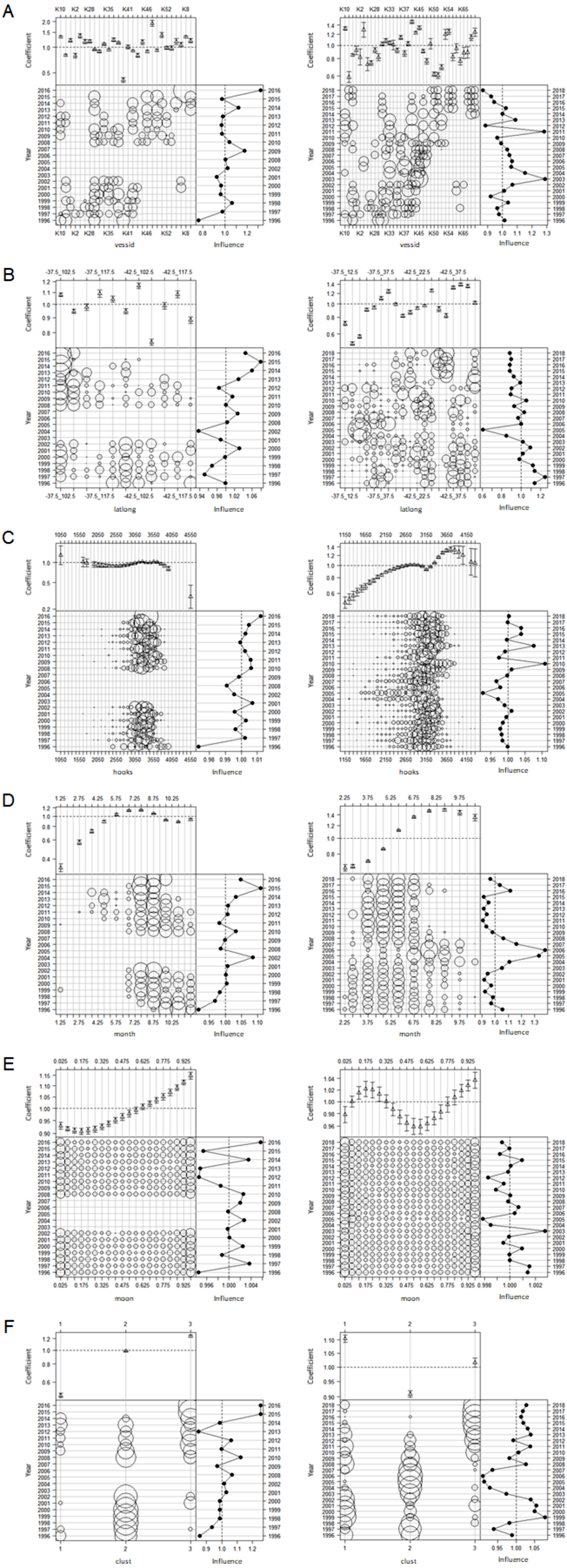
Vessel effects (Fig. 12A) were quite variable, with a few vessels having significantly lower or higher SBT catch rates. The influence changed through the time series, with the low number of vessels causing significant variability.
Spatial effects (Fig. 12B) showed significant variation in catch rates, with more variation in the statistical area 9 than area 8. In area 9 there was a trend towards fishing in areas with lower average catch rates. It would be useful to explore whether the areas of highest catch rate have moved through time. However, this would be difficult to determine from Korean data alone, since fishing activity is currently very concentrated spatially (Fig. 2). Given the behaviour of the species, areas of highest catch rate are also likely to move during the year, and we do not account for this in the model.
The effects of the number of hooks per set on catch rates (Fig. 12C) were difficult to interpret. In area 8 there were small differences by hook number across the range of data with most hooks, and minimal influence on year effects, apart from 2016 when effort was low and localized with only one vessel fishing. In area 9 there were relatively larger differences, and apparent influence on the year effects, with catchability averaging about 3% above the mean in 2010-16 (Fig. 12C). Sets with more than about 3,250 hooks tended to catch more SBT than sets with fewer hooks. In area 9 there were more sets with fewer hooks between 2004 and 2007, a period during which there were more zero SBT sets than at most other times (Fig. S2). These may reflect a mixture of targeting methods in area 9, with different fishing methods using different numbers of hooks.
Month effects (Fig. 12D) were strong in both areas 8 and 9, and relatively influential. In both areas, the highest catch rates were obtained in July and August, but slightly later in area 9. The seasonality of fishing effort changed through time, with the model suggesting that fishery timing increased mean catchability in the area 8 by over 10% higher than the average in 2015, and reduced it almost 5% below average in the area 9 in 2010-15.
Moon effects (Fig. 12E) showed that catch rates appeared to vary moderately with lunar illumination in area 8. In the area 9 delta lognormal models a similar effect was apparent in the lognormal positive component, but diminished overall by an inconclusive pattern in the binomial component (Fig. S8E).
The distribution of the cluster variable (Fig. 12F) changed considerably though time, as the behaviour of the fleet changed with the abundance of the target species. There were also relatively large differences in catch rate between the clusters, so this variable was quite influential on the indices, particularly in area 8.
Discussion
CPUE standardization in a multi-target fishery is more difficult than in a single target fishery, and various methods have been applied to differentiate fishing strategies through time (He, Bigelow & Boggs, 1997; Winker, Kerwath & Attwood, 2013; Winker, Kerwath & Attwood, 2014; Cosgrove et al., 2014; Thorson et al., 2017; Okamura et al., 2018).
In this study, abundance indices were derived from two alternative commonly used methods, data selection and cluster analysis, to explore how these approaches address target change through time.
The data selection method aims to identify effort targeted mostly at the target species, by selecting data based on fishing season, gear configuration, etc. This approach appeared to give reasonable results but was not entirely successful in accounting for the difference from nominal CPUE, as indicated by the high proportions of zero catches in the statistical area 8 in the early 2010s (Fig. S2).
Cluster analysis identifies target change through time based on species composition. In this study, cluster analysis appeared to be more useful than the data selection method, accounting better for the switch towards targeting ALB during the late 2000s in the area 9 and the early 2010s in the area 8 (Figs. S1 and S2). That is, the presence of more zero catches of SBT in the area 9 during the late 2000s and in area 8 during the early 2010s suggests that the data during those periods may include more effort targeted at other species, such as ALB. Since such contamination of the effort would tend to bias the indices, it is useful to separate sets with different fishing strategies. Applying cluster analysis to differentiate the fishing strategies may be the best approach for these periods. The clustering approach identified patterns that are consistent with our understanding of the fishery and changed the indices during those periods in a way that seems likely to better track the abundance.
Although we prefer the clustered data indices, the data selection method performed adequately. Thorough data exploration is needed to develop the selection criteria, and this process is perhaps the most useful part of the analysis. Data exploration provides the analyst with a good understanding of the structure of the fishery and how it has changed through time, and this understanding helps to shape the approaches used in the cluster analysis and generalized linear modelling.
A striking pattern emerging in the Korean tuna longline fishery is that the fleet has greatly concentrated its effort during the last five years. As SBT catch rates have increased, the fleet has significantly reduced the area fished to catch its quota, and in 2017 and 2018 its effort was more concentrated than ever before, with no effort in area 8. The Japanese longline fishery has also concentrated and reduced its effort in recent years (Itoh, 2019; Itoh & Takahashi, 2019), during which period the ‘Base’ abundance indices used as the primary indices for SBT in CCSBT have increased substantially. As such, similar recent trends of substantially increasing CPUE since the mid-2000s have been seen in both the Japanese and Korean longline fisheries (CCSBT, 2019a).
The indices estimated from the lognormal constant and the delta lognormal models were broadly similar for both approaches to address target change but differed somewhat more with the lognormal constant approach. The delta lognormal model in area 9 differed between unstandardized and standardized indices prior to 2005 and in recent years. The standardized indices were lower before 2005 mostly because of the change in spatial distribution. During that period, many fishing vessels that did not target SBT left the SBT fishing ground, so that a higher proportion of the remaining vessels targeted SBT (Fig. S3), and the cluster targeting variable reduced the level of the index (Fig. 12F). However, these changes were more than compensated for by the spatial effects, which tended to increase the standardized index prior to 2005. Similarly, the standardized area 9 indices in recent years were higher than the nominal indices, compared to the early to mid-2010s, because of increased effort in areas with (on average) lower catch rates due to slightly increased SBT quota. It is unclear why this has occurred, but it may be related to vessels avoiding the cost of moving to other areas, given that catch rates in all areas have risen in comparison to earlier years.
Reasons for the increasing effort concentration are not well understood, but several factors may be at play. Fishing is more efficient when catch rates are higher, and a vessel can catch its quota with fewer sets in a shorter period and smaller area. At higher abundance levels there may be also less requirement to move around and search for fish. Improving technology may also be having an impact. Increased availability of better information from oceanographic models and remote sensing data, and satellite communications, would reduce the amount of wasted effort due to fishing in areas with low SBT catch rates.
One effect of such increased effort concentration is loss of information for CPUE standardization, because effort occurs in fewer strata. This issue has caused problems in recent years for the main index of SBT abundance based on Japanese longline data (Itoh, 2020; Hoyle, 2020).
Catch rates varied with lunar illumination but this had little effect on the SBT index since effort was stable throughout each month (Fig. 12E). Longline catch rates of other pelagic fish such as bigeye tuna are known to be affected by moon phase (Poisson et al., 2010), but this has not previously been recorded for southern bluefin tuna. Southern bluefin tuna tend to swim deeper at night during the full moon (Bestley, Gunn & Hindell, 2009), and reduce the proportion of time spent near the surface at night as lunar illumination increases (Eveson et al., 2018), but it is unclear how this may affect catch rates. Similarly, Atlantic bluefin tuna (T. thynnus) swimming depth was significantly deeper around full moon (Wilson et al., 2005), although these effects differed by both location and season. The relationship between SBT catch rate and moon phase should be further investigated in the future, considering spatial and seasonal variation.
Like the abundance indices, the influence estimates are conditional on the model, which assumes no interactions between the different effects. Some interactions may be expected, such as variation between years in the timing and location of higher catch rates due to environmental variation affecting tuna movements. The small sample sizes limit the potential to model interaction terms, but there may be value in exploring space–time interactions using smoothing splines.
Fishing power has changed not only due to targeting strategy but also in association with vessel participation in the fishery through time, and these changes directly affect the catch rates of both target and bycatch species (Hoyle & Okamoto, 2011). Itoh & Takahashi (2019) took this effect into account when analyzing the index by selecting core vessels from the dataset. In this study, we applied all vessel data to the CPUE standardization models, and considered vessel effect (vessel identifier) as a categorical variable in the models. This effect was not very influential, apart from the early period when some vessels had significantly lower SBT catch rates. This is because in the early period there were some vessels that did not target SBT at the fishing grounds and fishing vessels targeting SBT have been there since around 2010 (Fig. S3). However, trends in fishing power estimated in this study represent the effects of changes in the fleet composition, but do not account for the changes caused by vessels that stay in the fishery and change their equipment or their fishing behaviour.
The Korean longline indices for SBT are not included in the stock assessment but intended for comparison with and corroboration of the primary index of abundance, which is based on the Japanese longline fishery. Analyses in two area-based components help to provide insight into spatial variation in the fishery and are also useful because seasonality varies by area.
Conclusion
The article compares two approaches, data selection and cluster analysis, for differentiating southern bluefin tuna (Thunnus maccoyii) targeting practices in the Korean tuna longline data and developing indices of relative abundance. In the case of Korean data, cluster analysis gave more reasonable results, but the data exploration required for the data selection method was invaluable in choosing the most appropriate method, and for understanding the structure of the fishery and how it has changed over time.
Supplemental Information
Mean catch per hundred hooks by year-quarter, species, and CCSBT statistical area (SA), plotted on a log scale, for albacore (ALB), yellowfin (YFT), bigeye (BET) and southern bluefin tuna (SBT)
Each CPUE has 1e−05 added so that zero catches appear on the log scale.
Proportion of zero catches per set by year-quarter, species, and CCSBT statistical area (SA), for albacore (ALB), yellowfin (YFT), bigeye (BET), and southern bluefin tuna (SBT)
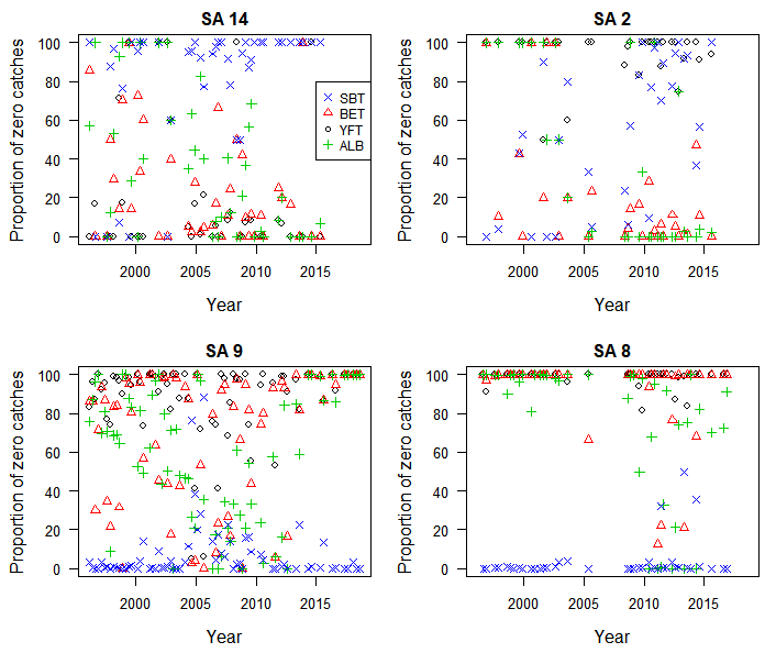
Plots of participation by vessel and year
Y axis represents a vessel, with the left plot sorted by the first year of participation, and the right plot sorted by the final year of participation.
Proportion of SBT in the total reported catch-in-numbers by 1° cell and month, aggregated over the period 1996–2018
Red colour indicates a higher proportion of SBT.
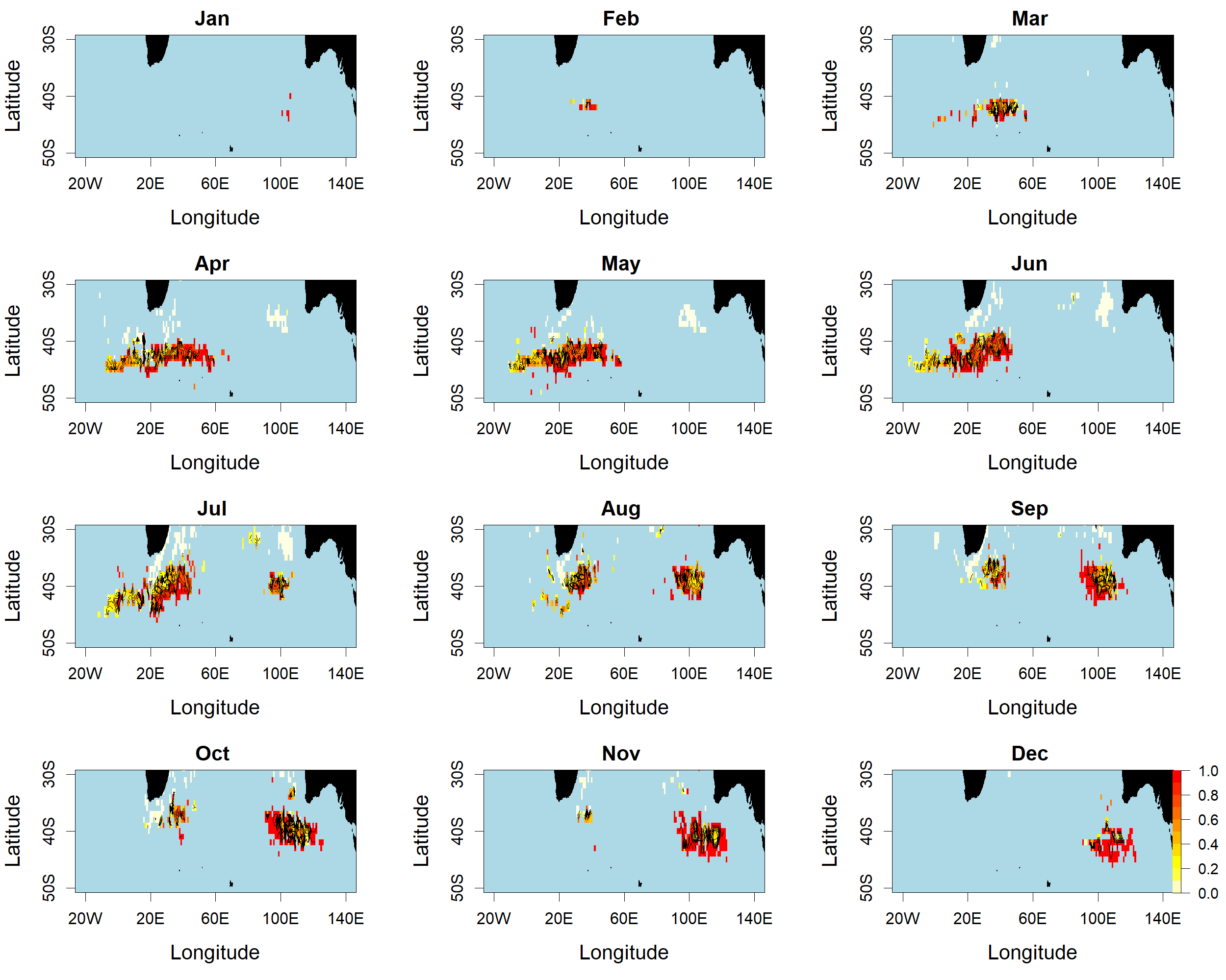
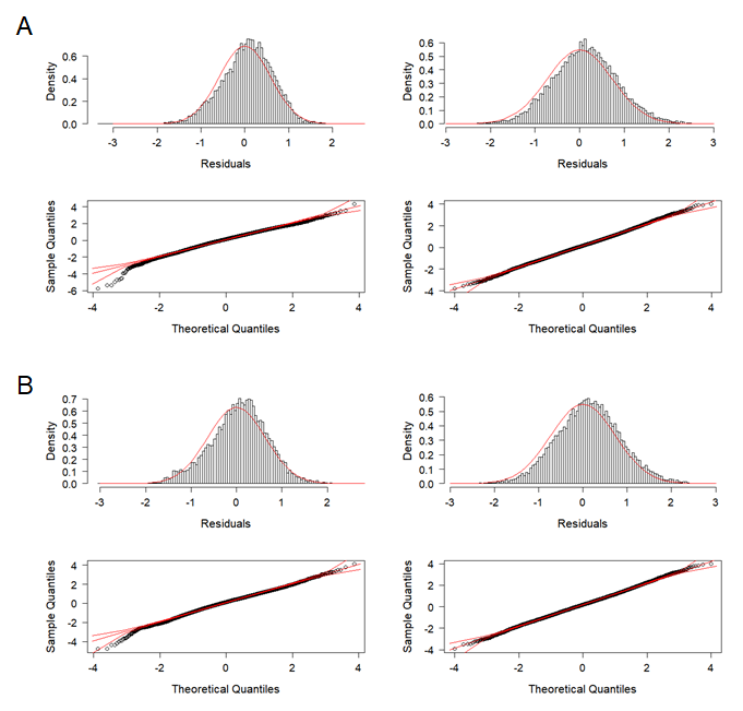
Frequency distributions of the standardized residuals and Q–Q plots of standardized residuals for lognormal constant models of CCSBT statistical areas 8 (left) and 9 (right), based on data selection and clustering analysis
(A) Data selection. (B) Clustering analysis.
Frequency distributions of the standardized residuals and Q-Q plots of standardized residuals for delta lognormal models of CCSBT statistical areas 8 (left) and 9 (right), based on data selection and clustering analysis
(A) Data selection. (B) Clustering analysis.
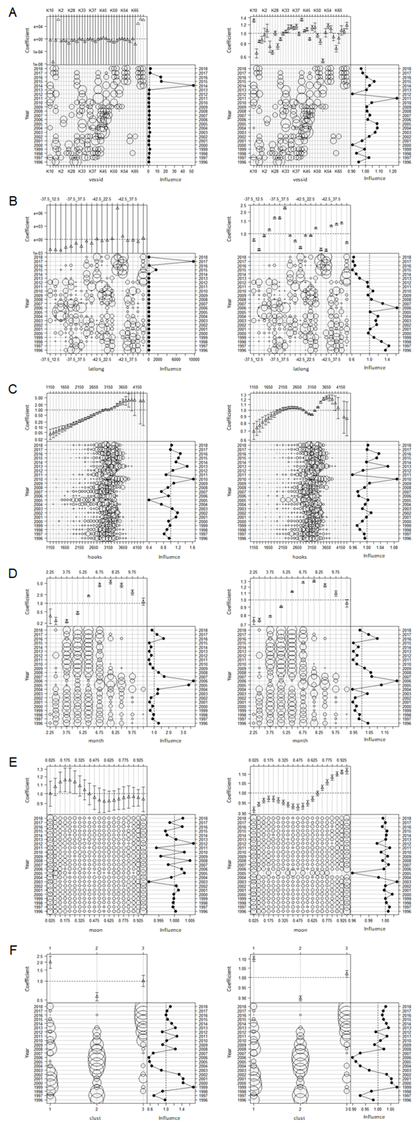
Influence plots for each effect for the binomial (left) and lognormal positive (right) components of delta lognormal model of CCSBT statistical areas 8, addressing target change using clustering
(A) Vessel effects. (B) Spatial (latlong) effects. (C) H ooks effects. (D) Month effects. (E) Moon effects. (F) Cluster effects.
Influence plots for each effect for the binomial (left) and lognormal positive (right) components of delta lognormal model of CCSBT statistical areas 9, addressing target change using clustering
(A) Vessel effects. (B) Spatial (latlong) effects. (C) Hooks effects. (D) Month effects. (E) Moon effects. (F) Cluster effects.