
Managing server clusters on intermittent power
- Published
- Accepted
- Received
- Academic Editor
- Srikumar Venugopal
- Subject Areas
- Distributed and Parallel Computing, Multimedia, Operating Systems
- Keywords
- Green data center, Intermittent power, Blink, Green cache, Memcached, Multimedia cache
- Copyright
- © 2015 Sharma et al.
- Licence
- This is an open access article distributed under the terms of the Creative Commons Attribution License, which permits unrestricted use, distribution, reproduction and adaptation in any medium and for any purpose provided that it is properly attributed. For attribution, the original author(s), title, publication source (PeerJ Computer Science) and either DOI or URL of the article must be cited.
- Cite this article
- 2015. Managing server clusters on intermittent power. PeerJ Computer Science 1:e34 https://doi.org/10.7717/peerj-cs.34
Abstract
Reducing the energy footprint of data centers continues to receive significant attention due to both its financial and environmental impact. There are numerous methods that limit the impact of both factors, such as expanding the use of renewable energy or participating in automated demand-response programs. To take advantage of these methods, servers and applications must gracefully handle intermittent constraints in their power supply. In this paper, we propose blinking—metered transitions between a high-power active state and a low-power inactive state—as the primary abstraction for conforming to intermittent power constraints. We design Blink, an application-independent hardware–software platform for developing and evaluating blinking applications, and define multiple types of blinking policies. We then use Blink to design both a blinking version of memcached (BlinkCache) and a multimedia cache (GreenCache) to demonstrate how application characteristics affect the design of blink-aware distributed applications. Our results show that for BlinkCache, a load-proportional blinking policy combines the advantages of both activation and synchronous blinking for realistic Zipf-like popularity distributions and wind/solar power signals by achieving near optimal hit rates (within 15% of an activation policy), while also providing fairer access to the cache (within 2% of a synchronous policy) for equally popular objects. In contrast, for GreenCache, due to multimedia workload patterns, we find that a staggered load proportional blinking policy with replication of the first chunk of each video reduces the buffering time at all power levels, as compared to activation or load-proportional blinking policies.
Introduction
Energy-related costs have become a significant fraction of total cost of ownership (TCO) in modern data centers. Recent estimates attribute 31% of TCO to both purchasing power and building and maintaining the power distribution and cooling infrastructure (Hamilton, 2010). Consequently, techniques for reducing the energy footprint of data centers continue to receive significant attention in both industry and the research community. We categorize these techniques broadly as being either primarily workload-driven or power-driven. Workload-driven systems reconfigure applications as their workload demands vary to use the least possible amount of power to satisfy demand (Ahmad & Vijaykumar, 2010; Moore, Chase & Ranganathan, 2006; Moore et al., 2005). In contrast, power-driven systems reconfigure applications as their power supply varies to achieve the best performance possible given the power constraints.
While prior work has largely emphasized workload-driven systems, power-driven systems are becoming increasingly important. For instance, data centers are beginning to rely on intermittent renewable energy sources, such as solar and wind, to partially power their operations (Gupta, 2010; Stone, 2007). Intermittent power constraints are also common in developing regions that experience “brownouts” where the electric grid temporarily reduces its supply under high load (Chase et al., 2001; Verma et al., 2009). The key challenge in power-driven systems is optimizing application performance in the presence of power constraints that may vary significantly and frequently over time. Importantly, these power and resource consumption constraints are independent of workload demands.
The ability to use intermittent power introduces other opportunities, beyond increasing use of renewable energy, for optimizing a data center to be cheaper, greener, and more reliable. We argue that designing systems to exploit these optimizations will move us closer to the vision of a net-zero data center.
-
Market-based electricity pricing. Electricity prices vary continuously based on supply and demand. Many utilities now offer customers access to market-based rates that vary every five minutes to an hour (Elevate Energy, 2011). As a result, the power data centers are able to purchase for a fixed price varies considerably and frequently over time. For instance, in the New England hourly wholesale market in 2011, maintaining a fixed $55/h budget, rather than a fixed per-hour power consumption, purchases 16% more power for the same price (Fig. 1). The example demonstrates that data centers that execute delay-tolerant workloads, such as data-intensive batch jobs, have an opportunity to reduce their electric bill by varying their power usage based on price.
-
Unexpected blackouts or brownouts. Data centers often use UPSs for backup power during unexpected blackouts. An extended blackout may force a data center to limit power consumption at a low level to extend UPS lifetime. While low power levels impact performance, it may be critical for certain applications to maintain some, even low, level of availability, e.g., disaster response applications. As we discuss, maintaining availability at low power levels is challenging if applications access distributed state. Further, in many developing countries, the electric grid is highly unstable with voltage rising and falling unexpectedly based on changing demands. These “brownouts” may also affect the power available to data centers over time.
-
100% power infrastructure utilization. Another compelling use of intermittent power is continuously operating a data center’s power delivery infrastructure at 100%. Since data center capital costs are enormous, maximizing the power delivery infrastructure’s utilization by operating as many servers as possible is important. However, data centers typically provision power for peak demands, resulting in low utilization (Fan, Weber & Barroso, 2007a; Kontorinis et al., 2012). In this case, intermittent power is useful to continuously run a background workload on a set of servers—designed explicitly for intermittent power—that always consume the excess power PDUs are capable of delivering. Since the utilization (and power usage) of a data center’s foreground workload may vary rapidly, the background servers must be capable of quickly varying power usage to not exceed the power delivery infrastructure’s limits.
In this paper, we present Blink, a new energy abstraction for gracefully handling intermittent power constraints. Blinking applies a duty cycle to servers that controls the fraction of time they are in the active state, e.g., by activating and deactivating them in succession, to gracefully vary their energy footprint. For example, a system that blinks every 30 s, i.e., is on for 30 s and then off for 30 s, consumes half the energy, modulo overheads, of an always-on system. Blinking generalizes the extremes of either keeping a server active (a 100% duty cycle) or inactive (a 0% duty cycle) by providing a spectrum of intermediate possibilities. Blinking builds on prior work in energy-aware design. First, several studies have shown that turning a server off when not in use is the most effective method for saving energy in server clusters (Chase et al., 2001; Pinheiro et al., 2001). Second, blinking extends the PowerNap (Meisner, Gold & Wenisch, 2009) concept, which advocates frequent transitions to a low-power sleep state, as an effective means of reducing idle power waste.
An application’s blinking policy decides when each node is active or inactive at any instant based on both its workload characteristics and energy constraints. Clearly, blinking impacts application performance, since there may not always be enough energy to power the nodes necessary to meet demand. Hence, the goal of a blinking policy is to minimize performance degradation as power varies. In general, application modifications are necessary to adapt traditional server-based applications for blinking, since these applications implicitly assume always-on, or mostly-on, servers. Blinking forces them to handle regular disconnections more often associated with weakly connected (Terry et al., 1995) environments, e.g., mobile, where nodes are unreachable whenever they are off or out of range.
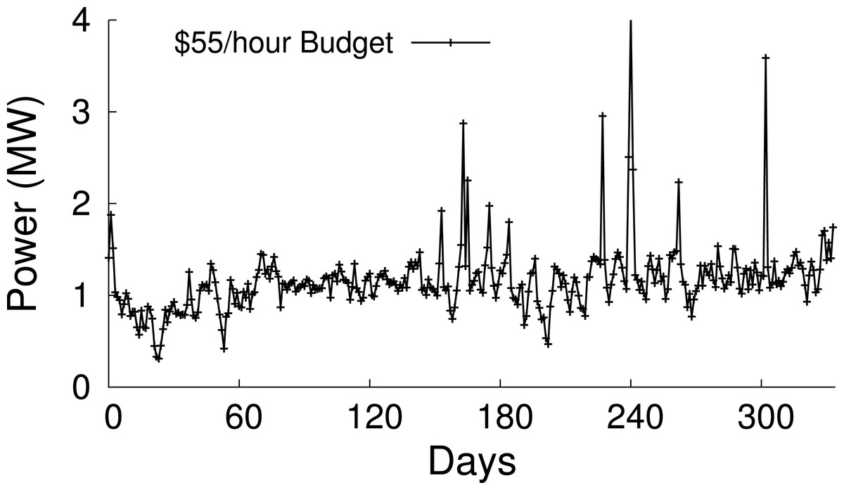
Figure 1: Electricity prices vary every five minutes to an hour in wholesale markets, resulting in the power available for a fixed monetary budget varying considerably over time
Example applications for blink
To demonstrate how blinking impacts common data center applications, we explore the design of BlinkCache—a blinking version of memcached that gracefully handles intermittent power constraints and GreenCache—a distributed cache for multimedia data that runs off renewable energy—as proof-of-concept examples.
Memcached is a distributed memory cache for storing key-value pairs that many prominent Internet sites, including LiveJournal, Facebook, Flickr, Twitter, YouTube, and others, use to improve their performance. For Internet services that store user-generated content, the typical user is often interested in the relatively unpopular objects in the heavy tail, since these objects represent either their personal content or the content of close friends and associates. As one example, Fig. 2 depicts a popularity distribution for Facebook group pages in terms of their number of fans. While the figure only shows the popularity rank of the top 10,000 pages, Facebook has over 20 million group pages in total. Most of these pages are nearly equally unpopular. For these equally unpopular objects, blinking nodes synchronously to handle variable power constraints results in fairer access to the cache because the probability of finding an object becomes equal for all objects in the cache. While fair cache access is important, maximizing memcached’s hit rate requires prioritizing access to the most popular objects. We explore these performance tradeoffs in-depth for a memcached cluster with intermittent power constraints.
In contrast, GreenCache leverages the blinking abstraction to modulate its energy footprint to match available power while minimizing both backhaul bandwidth and client access latency for a large video library. As discussed above, minimizing bandwidth usage (or cost) and maximizing users’ experience, e.g., by reducing buffering time, are the two primary goals of a multimedia cache. We analyze video traffic behavior of a large number of users for the most popular user-generated video site, YouTube, and exploit traffic characteristics and video properties to design new placement and blinking policies for minimizing bandwidth usage and maximizing users’ experience.
Contributions
In designing, implementing, and evaluating BlinkCache and GreenCache as proof-of-concept examples of using the blink abstraction, this paper makes the following contributions.1
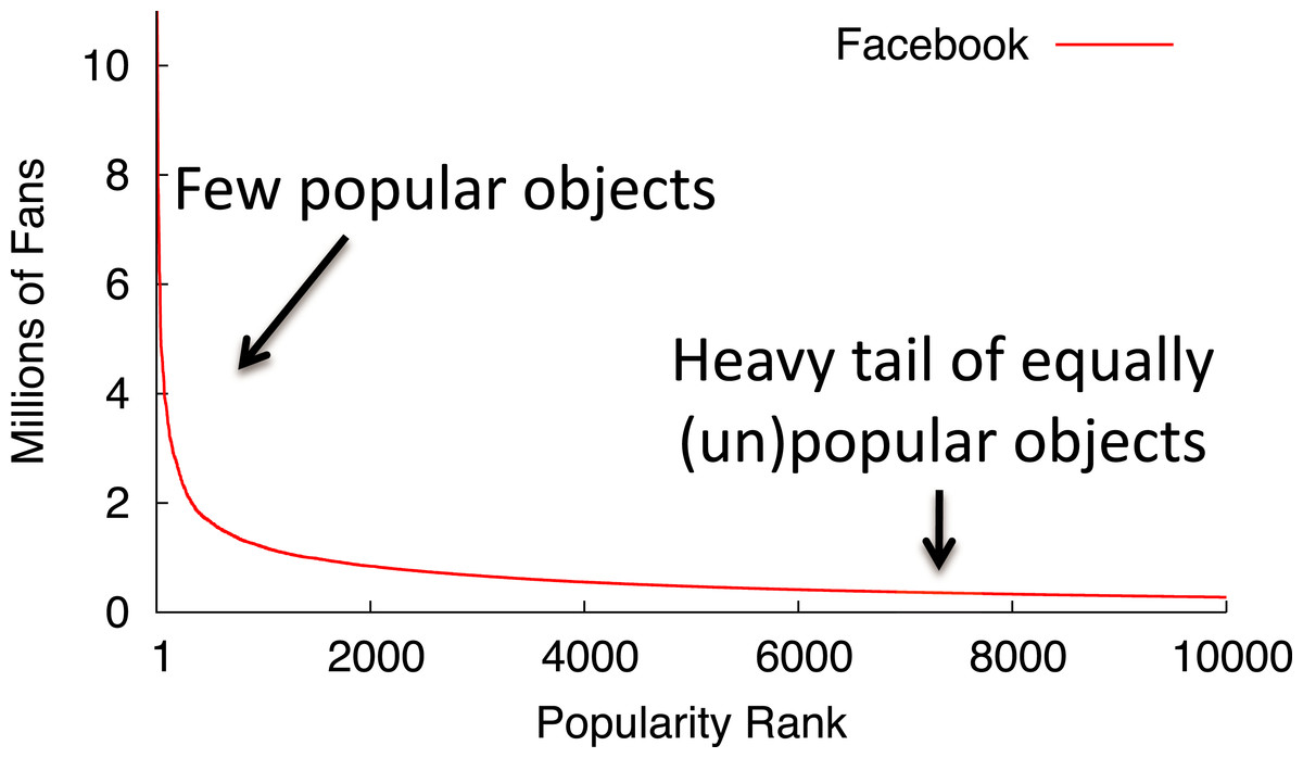
Figure 2: The popularity of web data often exhibits a long heavy tail of equally unpopular objects.
This graph ranks the popularity of Facebook group pages by their number of fans.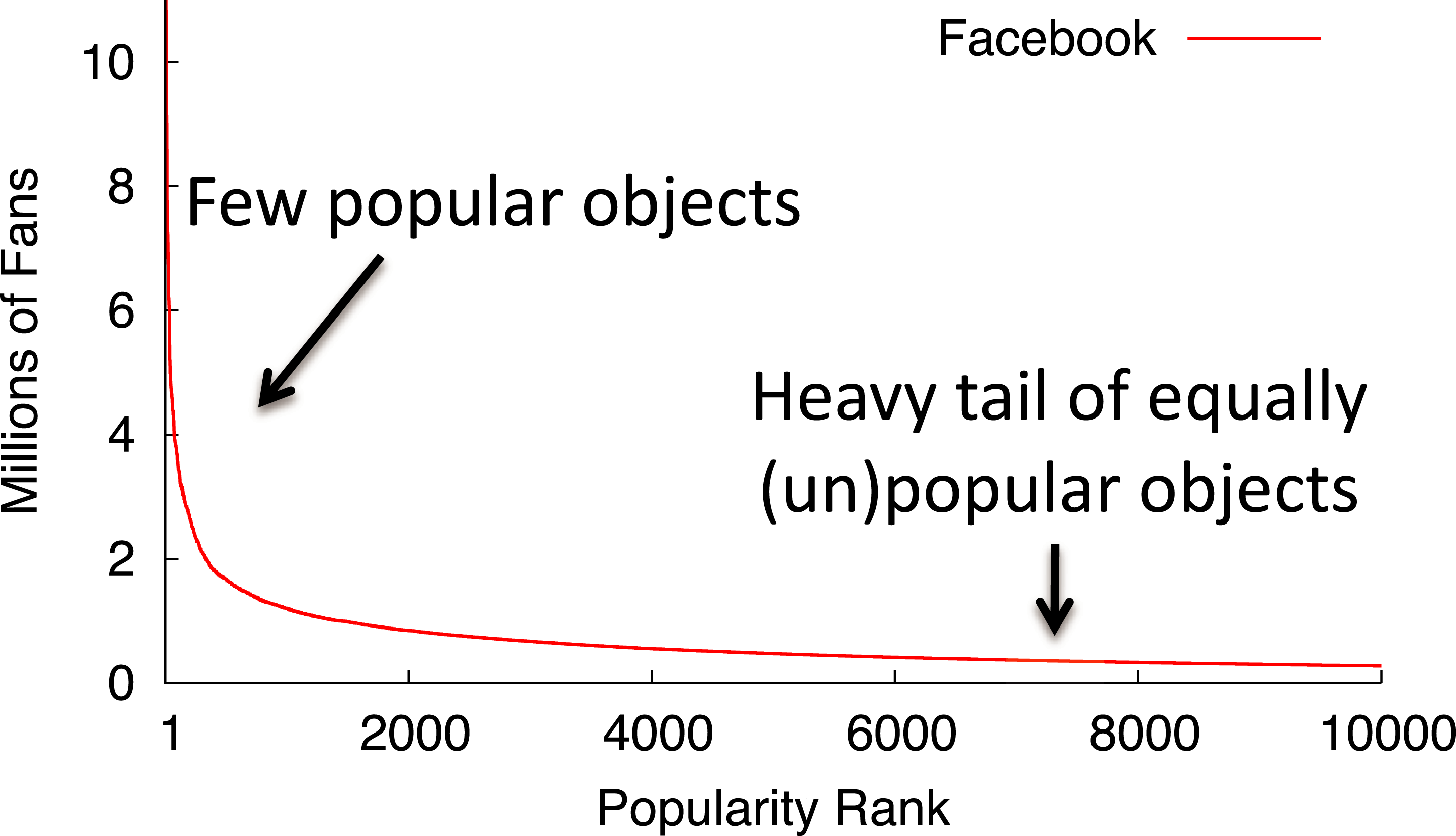
-
Make the case for blinking systems. We propose blinking systems to deal with variable power constraints in server clusters. We motivate why blinking is a beneficial abstraction for dealing with intermittent power constraints, define different types of blinking policies, and discuss its potential impact on a range of distributed applications.
-
Design a blinking hardware/software platform. We design Blink, an application-independent hardware/software platform to develop and evaluate blinking applications. Our small-scale prototype uses a cluster of 10 low-power motherboards connected to a programmable power meter that replays custom power traces and variable power traces from a solar and wind energy harvesting deployment.
-
Design, Implement, Evaluate BlinkCache and GreenCache. We use Blink to experiment with blinking policies for BlinkCache and GreenCache, a variant of memcached and multimedia cache, respectively, and optimize the performance for intermittent power constraints. For BlinkCache, our hypothesis is that a load-proportional blinking policy, which keeps nodes active in proportion to the popularity of the data they store, combined with object migration to group together objects with similar popularities, results in near optimal cache hit rates, as well as fairness for equally unpopular objects. To validate our hypothesis, we compare the performance of activation, synchronous, and load-proportional policies for realistic Zipf-like popularity distributions. We show that a load-proportional policy is significantly more fair than an optimal activation policy for equally popular objects (4X at low power) while achieving a comparable hit rate (over 60% at low power). For GreenCache, our hypothesis is that a staggered load proportional policy which keeps the nodes active based on their load and the available power in staggered manner, with replication of the first chunk of each video on all servers, yields lower buffering time for clients, compared to activation or load-proportional blinking policies, when operating under variable power.
-
Blinking scalability performance. To see how blinking scales with the size of a cluster we emulate our small-scale server cluster and study the performance of BlinkCache and GreenCache for a 1,000 node cluster. Our hypothesis is that the performance of a blinking policy should be independent of the cluster size.
‘Blink: Rationale and Overview’ provides an overview of the blinking abstraction and various blinking policies. ‘Blink Prototype’ presents Blink’s hardware and software architecture in detail, while ‘BlinkCache: Blinking Memcached’ presents design alternatives for BlinkCache, a blinking version of memcached. ‘GreenCache: Blinking Multimedia Cache’ presents the design techniques for GreenCache, a blinking version of multimedia cache. We provide the implementation and evaluation of both applications in ‘Implementation’ and ‘Evaluation’, respectively. Finally, ‘Related Work’ discusses related work, ‘Applicability of Blinking’ outlines the applicability of blinking to other applications, and ‘Conclusion’ concludes.
Blink: Rationale and Overview
Today’s computing systems are not energy-proportional (Barroso & Hölzle, 2007)—a key factor that hinders data centers from effectively varying their power consumption by controlling their utilization. Designing energy-proportional systems is challenging, in part, since a variety of server components, including the CPU, memory, disk, motherboard, and power supply, now consume significant amounts of power. Thus, any power optimization that targets only a single component is not sufficient for energy-proportionality, since it reduces only a fraction of the total power consumption (Barroso & Hölzle, 2007; Le Sueur & Heiser, 2010). As one example, due to the power consumption of non-CPU components, a modern server that uses dynamic voltage and frequency scaling in the CPU at low utilization may still operate at over 50% of its peak power (Anderson et al., 2009; Tolia et al., 2008). Thus, deactivating entire servers, including most of their components, remains the most effective technique for controlling energy consumption in server farms, especially at low power levels that necessitate operating servers well below 50% peak power on average.
However, data centers must be able to rapidly activate servers whenever workload demand increases. PowerNap (Meisner, Gold & Wenisch, 2009) proposes to eliminate idle power waste and approximate an energy-proportional server by rapidly transitioning the entire server between a high-power active state and a low-power inactive state. PowerNap uses the ACPI S3 state, which places the CPU and peripheral devices in sleep mode but preserves DRAM memory state, to implement inactivity. Transition latencies at millisecond-scale, or even lower, may be possible between ACPI’s fully active S0 state and its S3 state. By using S3 to emulate the inactive “off” state.2 PowerNap is able to consume minimal energy while sleeping. Typical high-end servers draw as much as 40× less power in S3.
Blink extends PowerNap in important ways. First, PowerNap is a workload-driven technique that eliminates idle server power waste—it uses rapid transitions in a workload-driven fashion to activate each server when work arrives and deactivate it when idle. In contrast, Blink is a power-driven technique that regulates average node power consumption independent of workload demands. Second, the PowerNap mechanism applies to each server independently, while Blink applies to collections of servers. Blinking policies, which we formally define next, are able to capture, and potentially exploit, cross-server dependencies and correlations in distributed applications. Finally, unlike workload-driven transitions, blinking provides benefits even for the non-ideal S3 transition latencies on the order of seconds that are common in practice, as we show in ‘Balancing performance and fairness.’3 Table 1 shows S3 transition latencies for a variety of platforms, as reported in Agarwal et al. (2009), with the addition of Blink’s OLPC-X0 nodes. The latencies include both hardware transitions, as well as the time to restart the OS and reset its IP address.
| Type | Model | S3 transition time (s) |
|---|---|---|
| Desktop | Optiplex 745 | 13.8 |
| Desktop | Dimension 4600 | 12.0 |
| Laptop | Lenovo X60 | 11.7 |
| Laptop | Lenovo T60 | 9.7 |
| Laptop | Toshiba M400 | 9.1 |
| Laptop | OLPC-XO (w/NIC) | 1.6 |
| Laptop | OLPC-XO (no NIC) | 0.2 |
The blink state of each node i is defined by two parameters that determine its duty cycle di, (i) length of the ON interval ton and (ii) length of the OFF interval toff, such that
A blink policy defines the blink state of each node in a cluster, as well as a blink schedule for each node.
The blink schedule defines the clock time at which a specified node transitions its blink state to active, which in turn dictates the time at which the node turns on and goes off. The schedule allows nodes to synchronize their blinking with one another, where appropriate. For example, if node A frequently accesses disk files stored on node B, the blink policy should specify a schedule such that the nodes synchronize their active intervals. To illustrate how a data center employs blinking to regulate its aggregate energy usage, consider a scenario where the energy supply is initially plentiful and there is sufficient workload demand for all nodes. In this case, a feasible policy is to keep all nodes continuously on.
Next assume that the power supply drops by 10%, and hence, the data center must reduce its aggregate energy use by 10%. There are several blinking policies that are able to satisfy this 10% drop. In the simplest case, 10% of the nodes are turned off, while the remaining nodes continue to stay on. Alternatively, another blinking policy may specify a duty cycle of di = 90% for every node i. There are also many ways to achieve a per-server duty cycle of 90% by setting different ton and toff intervals, e.g., ton = 9 s and toff = 1 s or ton = 900 ms and toff = 100 ms. Yet another policy may assign different blink states to different nodes, e.g., depending on their loads, such that aggregate usage decreases by 10%.
We refer to the first policy in our example above as an activation policy. An activation policy only varies the number of active servers at each power level (Chase et al., 2001; Tolia et al., 2008), such that some servers are active, while others are inactive; the energy supply dictates the size of the active server set. In contrast, synchronous policies toggle all nodes between the active and inactive state in tandem. In this case, all servers are active for ton seconds and then inactive for toff seconds, such that total power usage over each duty cycle matches the available power. Of course, since a synchronous policy toggles all servers to active at the same time, it does not reduce peak power, which has a significant impact on the cost of energy generation. An asynchronous policy may randomize the start of each node’s active interval to decrease peak power without changing the average power consumption across all nodes. In contrast to an asynchronous policy, an asymmetric policy may blink different nodes at different rates, while ensuring the necessary change in the energy footprint. For example, an asymmetric policy may be load-proportional and choose per-node blink states that are a function of current load. Finally, a staggered blinking policy is a type of asynchronous policy that staggers the start time of all nodes equally across each blink interval. A staggered policy that reduces the energy footprint by blinking nodes in proportion to the current load at each node is called staggered load-proportional policy.
Blink and blink policies are designed to cap power consumption of a server cluster to the power supply. All of the policies above are equally effective at capping the average power consumption for a variable power signal over any time interval. However, the choice of the blink policy greatly impacts application performance. Although Blink’s design is application-independent, applications should be modified and made blink-aware to perform well on a blinking cluster. In this paper, we design blinking policies for two specific types of distributed applications—BlinkCache, a blinking version of memcached and GreenCache, a blinking version of multimedia cache. In designing these policies, we profile application performance for a variety of blinking policies when subjected to different changes in available power. Our goal in this paper is to demonstrate the feasibility of running distributed applications while performing well under extreme power constraints; optimizing performance for any specific workload and QOS demands is beyond the scope of this paper.
Blink Prototype
Blink is a combined hardware/software platform for developing and evaluating blinking applications. This section describes our prototype’s hardware and software architecture in detail.
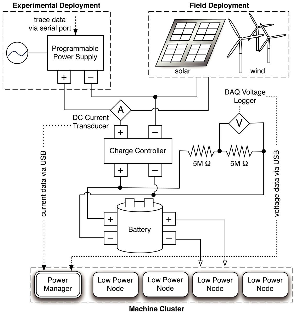
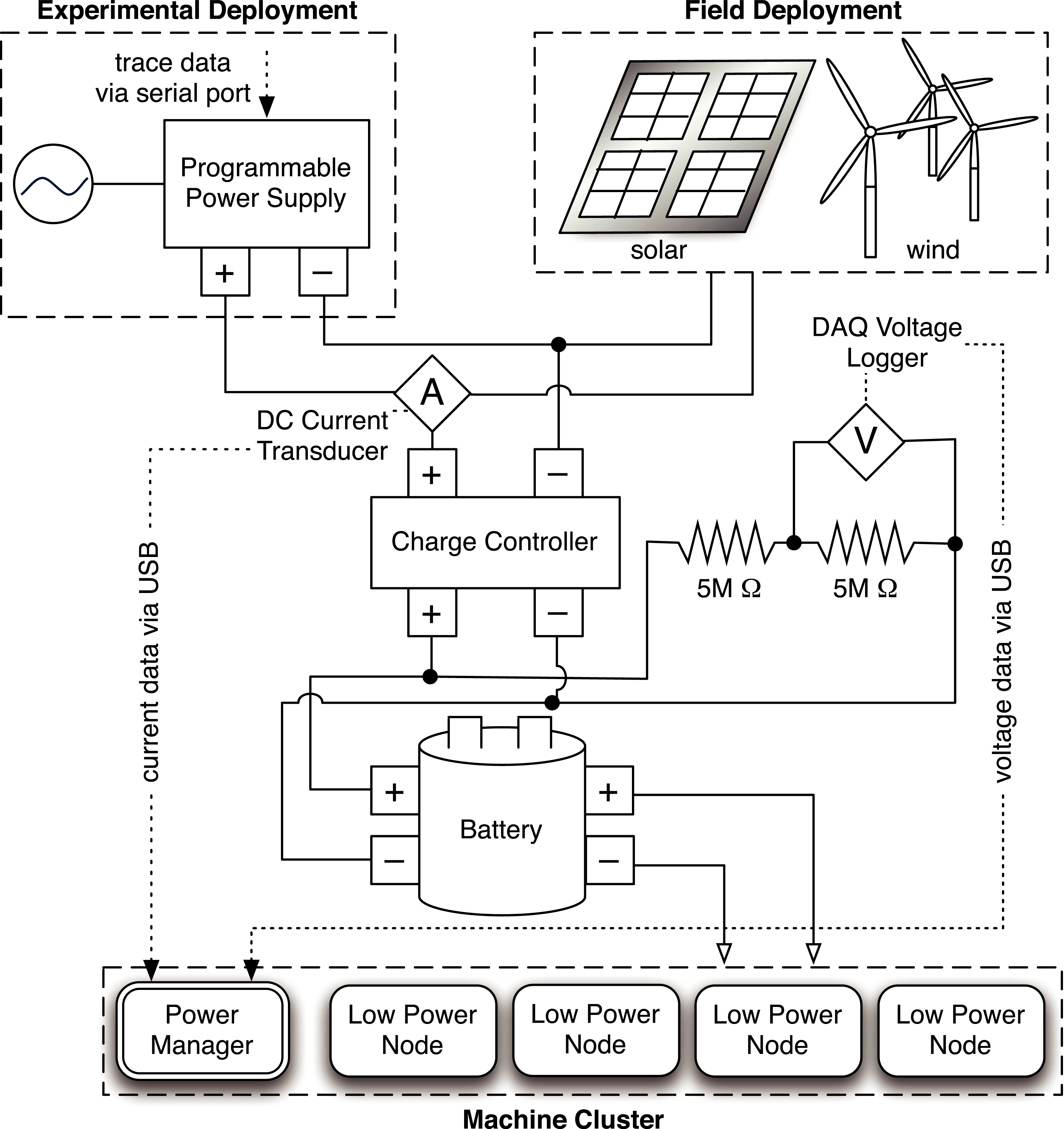
Figure 3: Hardware architecture of the Blink prototype.
Blink hardware platform
Blink’s current hardware platform consists of two primary components: (i) a low-power server cluster that executes Blink-aware applications and (ii) a variable energy source constructed using an array of micro wind turbines and solar panels. We use renewable energy to expose the cluster to intermittent power constraints.
Energy sources
We deployed an array of two wind turbines and two solar panels to power Blink. Each wind turbine is a SunForce Air-X micro-turbine designed for home rooftop deployment, and rated to produce up to 400 W in steady 28 mph winds. However, in our measurements, each turbine generates approximately 40 W of power on windy days. Our solar energy source uses Kyocera polycrystalline solar panels that are rated to produce a maximum of 65 W at 17.4 V under full sunlight. Although polycrystalline panels are known for their efficiency, our measurements show that each panel only generates around 30 W of power in full sunlight and much less in cloudy conditions.
We assume blinking systems use batteries for short-term energy storage and power buffering. Modern data centers and racks already include UPS arrays to condition power and tolerate short-term grid disruptions. We connect both renewable energy sources in our deployment to a battery array that includes two rechargeable deep-cycle ResourcePower Marine batteries with an aggregate capacity of 1,320 watt-hours at 12 V, which is capable of powering our entire cluster continuously for over 14 h. However, in this paper we focus on energy-neutral operation over short time intervals, and thus use the battery array only as a small 5-minute buffer. We connect the energy sources to the battery pack using a TriStar T-60 charge controller that provides over-charging circuitry. We deployed our renewable energy sources on the roof of a campus building and used a HOBO U30 data logger to gather detailed traces of current and voltage over a period of several months under a variety of different weather conditions.
While our energy harvesting deployment is capable of directly powering Blink’s server cluster, to enable controlled and repeatable experiments we leverage four Extech programmable power supplies. We use the programmable power supplies, instead of the harvesting deployment, to conduct repeatable experiments by replaying harvesting traces, or emulating other intermittent power constraints, to charge our battery array.4
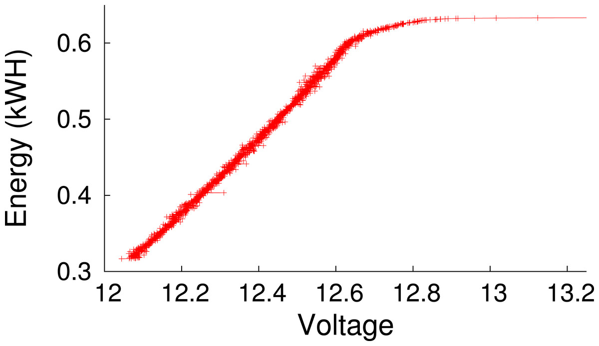
Figure 4: Empirically-measured battery capacity as a function of voltage for our deep-cycle battery.
We consider the battery empty below 12 V, since using it beyond this level will reduce its lifetime.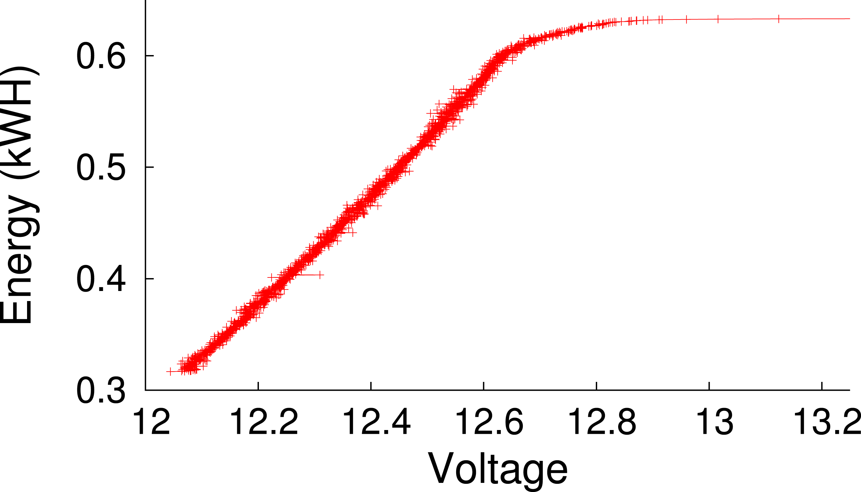
Since the battery’s voltage level indicates its current energy capacity, we require sensors to measure and report it. We use a data acquisition device (DAQ) from National Instruments to facilitate voltage measurement. As shown in Fig. 3, the prototype includes two high-precision 5MOhm resistors between the battery terminals and employs the DAQ to measure voltage across each resistor. We then use the value to compute the instantaneous battery voltage, and hence, capacity. Figure 4 shows the empirically-derived capacity of our prototype’s battery as a function of its voltage level. In addition to battery voltage, we use DC current transducers to measure the current flowing from the energy source into the battery, and the current flowing from the battery to the cluster. The configuration allows Blink to accurately measure these values every second.
Low-power server cluster
Our Blink prototype uses a cluster of low-power server nodes. To match the energy footprint of the cluster with the power output of our energy harvesting deployment we construct our prototype from low-power nodes that use AMD Geode processor motherboards. Each motherboard, which we scavenge from OLPC-XO laptops, consists of a 433 MHz AMD Geode LX CPU, 256 MB RAM, a 1GB solid-state flash disk, and a Linksys USB Ethernet NIC. Each node runs the Fedora Linux distribution with kernel version 2.6.25. We connect our 10 node cluster together using an energy-efficient switch (Netgear GS116) that consumes 15 W. Each low-power node consumes a maximum of 8.6 W, and together with the switch, the 10 node cluster has a total energy footprint of around 100 W. An advantage of using XO motherboards is that they are specifically optimized for rapid S3 transitions that are useful for blinking. Further, the motherboards use only 0.1 W in S3 and 8.6 W in S0 at full processor and network utilization. The wide power range in these two states combined with the relatively low power usage in S3 makes these nodes an ideal platform for demonstrating the efficacy of Blink’s energy optimizations.
Though XO motherboards are energy-efficient and consume little power even at full utilization they are not suitable for running applications which require large persistent storage, such as a multimedia cache. The same design also scales to more powerful servers. As a result, for our multimedia cache application, we design a Blink-aware cluster, but we replace XO motherboards with Mac minis. Each Mac mini consists of a 2.4 GHz Intel Core 2 Duo processors, 2 GB RAM, and a 40 GB flash-based SSD. We boot each Mac mini in text mode and unload all unnecessary drivers in order to minimize the time it takes to transition into S3. With the optimizations, the time to transition to and from ACPI’s S3 state on the Mac mini is one second, and the power consumption in S3 and S0 is 1 W and 25 W respectively.
Blink software architecture
Blink’s software architecture consists of an application-independent control plane that combines a power management service with per-node access to energy and node-level statistics. Blink-aware applications interact with the control plane using Blink APIs to regulate their power consumption. The power management service consists of a power manager daemon that runs on a gateway node and a power client daemon that runs on each cluster node. The architecture separates mechanism from policy by exposing a single simple interface for applications to control blinking for each cluster node.
| Blinking interface |
|---|
| setDutyCycle(int nodeId, int onPercentage) |
| setBlinkInterval(int nodeId, int interval) |
| syncActiveTime(int node, long currentTime) |
| forceSleep(int nodeId, int duration) |
| Measurement interface |
|---|
| getBatteryCapacity() |
| getBatteryEnergy() |
| getChargeRate(int lastInterval) |
| getDischargeRate(int lastInterval) |
| getServerLoadStats(int nodeId) |
The power manager daemon has access to the hardware sensors, described above, that monitor the battery voltage and current flow. Each Blink power client also monitors host-level metrics on each cluster node and reports them to the power manager. These metrics include CPU utilization, network bandwidth, and the length of the current active period. The power client exposes an internal RPC interface to the power manager that allows it to set a node’s blinking pattern. To set the blinking pattern, the power client uses the timer of the node’s real-time clock (RTC) to automatically sleep and wake up, i.e., transition back to S0, at specific intervals. Thus, the power client is able to set repetitive active and inactive durations. For example, the power manager may set a node to repeatedly be active for 50 s and inactive for 10 s. In this case, the blink interval is 60 s with the node being active 83% of the time and inactive 17% of the time. We assume that nodes synchronize clocks using a protocol, such as NTP, to enable policies that coordinate blink schedules across cluster nodes.
The impact of clock synchronization is negligible for our blink intervals at the granularity of seconds, but may become an issue for blink intervals at the granularity of milliseconds or less. Note that clock synchronization is not an issue for applications, such as memcached, that do not perform inter-node communication. Transitioning between S0 and S3 incurs a latency that limits the length of the blink interval. Shorter blink intervals are preferable since they allow each node to more closely match the available power, more rapidly respond to changes in supply, and reduces the battery capacity necessary for short term buffering. The XO motherboard yields S3 sleep latencies that range from roughly 200 ms to 2 s depending on the set of active devices and drivers (see Table 1). For instance, since our USB NIC driver does not implement the ACPI reset_resume function, we must unload and load its driver when transitioning to and from S3. As a result, the latency for XO motherboard is near 2 s. Similarly, with similar optimizations, the time to transition to and from ACPI’s S3 state on the Mac mini is 1 s. Unfortunately, inefficient and incorrect device drivers are commonplace, and represent one of the current drawbacks to blinking in practice.
The Blink control plane exposes an RPC interface to integrate with external applications as shown in Tables 2 and 3. Applications use these APIs to monitor input/output current flow, battery voltage, host-level metrics and control per-node blinking patterns. Since Blink is application-independent, the prototype does not report application-level metrics.
BlinkCache: Blinking Memcached
Memcached is a distributed in-memory cache for storing key-value pairs that significantly reduces both the latency to access data objects and the load on persistent disk-backed storage. Memcached has become a core component in Internet services that store vast amounts of user-generated content, with services maintaining dedicated clusters with 100s to 1,000s of nodes (Ousterhout et al., 2009). Since end users interact with these services in real-time through web portals, low-latency access to data is critical. High page load latencies frustrate users and may cause them to stop generating new content (Nah, 2004), which is undesirable since these services’ primary source of revenue derives from their content, e.g., by selling targeted ads.
Memcached overview
Memcached’s design uses a simple and scalable client-server architecture, where clients request a key value directly from a single candidate memcached server with the potential to store it. Clients use a built-in mapping function to determine the IP address of this candidate server. Initial versions of memcached determined the server using the function Hash(Key)%NumServers, while the latest versions use the same consistent hashing approach popularized in DHTs, such as Chord (Stoica et al., 2001). In either case, the key values randomly map to nodes without regard to their temporal locality, i.e., popularity. Since all clients use the same mapping function, they need not communicate with other clients or servers to compute which server to check for a given key. Likewise, Memcached servers respond to client requests (gets and sets) without communicating with other clients or servers. This lack of inter-node communication enables Memcached to scale to large clusters.
Importantly, clients maintain the state of the cache, including its consistency with persistent storage. As a result, applications are explicitly written to use memcached by (i) checking whether an object is resident in the cache before issuing any subsequent queries, (ii) inserting a newly referenced object into the cache if it is not already resident, and (iii) updating a cached object to reflect a corresponding update in persistent storage. Each memcached server uses the Least Recently Used (LRU) replacement policy to evict objects. One common example of a cached object is an HTML fragment generated from the results of multiple queries to a relational database and other services. Since a single HTTP request for many Internet services can result in over 100 internal, and potentially sequential, requests to other services (DeCandia et al., 2007; Ousterhout et al., 2009), the cache significantly decreases the latency to generate the HTML.
Access patterns and performance metrics
The popularity of web sites has long been known to follow a Zipf-like distribution (Breslau et al., 1999; Wolman et al., 1999), where the fraction of all requests for the ith most popular document is proportional to 1/iα for some constant α. Previous studies (Breslau et al., 1999; Wolman et al., 1999) have shown that α is typically less than one for web site popularity. The key characteristic of a Zipf-like distribution is its heavy tail, where a significant fraction of requests are for relatively unpopular objects. We expect the popularity of user-generated content for an Internet service to be similar to the broader web, since, while some content may be highly popular, such as a celebrity’s Facebook page, most users are primarily interested in either their own content or the content of close friends and associates.
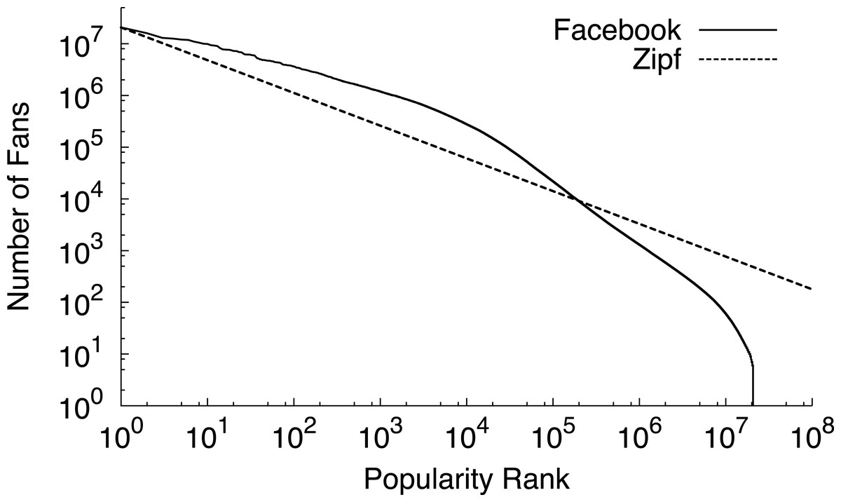
Figure 5: The popularity rank, by number of fans, for all 20 million public group pages on Facebook follows a Zipf-like distribution with α = 0.6.
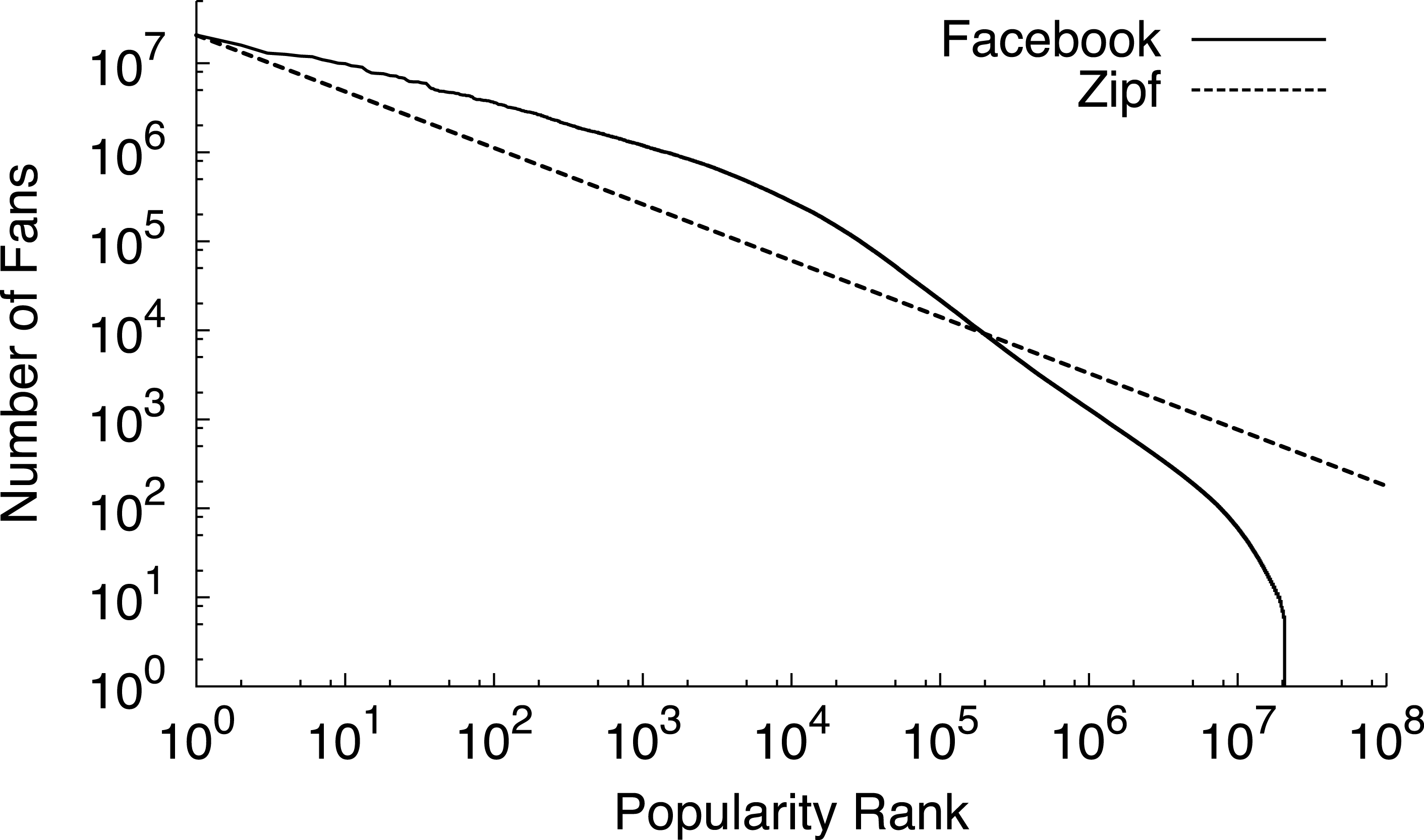
As a test of our expectation, we rank all 20 million user-generated fan pages on Facebook by their number of fans. We use the size of each page’s fan base as a rough approximation of the popularity of its underlying data objects. Figure 5 confirms that the distribution is Zipf-like with α approximately 0.6. Recent work also states that Facebook must store a significant fraction of their data set in massive memcached clusters, i.e., on the order of 2,000 nodes, to achieve high hit rates, e.g., 25% of the entire data set to achieve a 96.5% hit rate (Ousterhout et al., 2009). This characteristic is common for Zipf-like distributions with low α values, since many requests for unpopular objects are inside the heavy tail. Thus, the distribution roughly divides objects into two categories: the few highly popular objects and the many relatively unpopular objects. As cache size increases, it stores a significant fraction of objects that are unpopular compared to the few popular objects, but nearly uniformly popular compared to each other. These mega-caches resemble a separate high-performance storage tier (Ousterhout et al., 2009) for all data objects, rather than a small cache for only the most popular data objects.
Before discussing different design alternatives for BlinkCache, we define our performance metrics. The primary cache performance metric is hit ratio, or hit rate, which represents the percentage of object requests that the cache services. A higher hit rate indicates both a lower average latency per request, as well as lower load on the back-end storage system. In addition to hit rate, we argue that fairness should be a secondary performance metric for large memcached clusters that store many objects of equal popularity. A fair cache distributes its benefits—low average request latency—equally across objects. Caches are usually unfair, since their primary purpose is to achieve high hit rates by storing more popular data at the expense of less popular data. However, fairness increases in importance when there are many objects with a similar level of popularity, as in today’s large memcached clusters storing data that follows a Zipf-like popularity distribution. An unfair cache results in a wide disparity in the average access latency for these similarly popular objects, which ultimately translates to end-users receiving vastly different levels of performance. We use the standard deviation of average request latency per object as our measure of fairness. The lower the standard deviation the more fair the policy, since this indicates that objects have average latencies that are closer to the mean.
BlinkCache design alternatives
We compare variants of three basic memcached policies for variable power constraints: an activation policy, a synchronous policy, and an asymmetric load-proportional policy. In all cases, any get request to an inactive server always registers as a cache miss, while any set request is deferred until the node becomes active. We defer a discussion of the implementation details using Blink to the next section.
-
Activation policy. An activation policy ranks servers 1…N and always keeps the top M servers active, where M is the maximum number of active servers the current power level supports. We discuss multiple activation variants, including a static variant that does not change the set of available servers in each client’s built-in mapping function to reflect the current set of active servers, and a dynamic variant that does change the set. We also discuss a key migration variant that continuously ranks the popularity of objects and migrates them to servers 1…N in rank order.
-
Synchronous policy. A synchronous policy keeps all servers active for time t and inactive for time T − t for every interval T, where t is the maximum duration the current power level supports and T is short enough to respond to power changes but long enough to mitigate blink overhead. The policy does not change the set of available servers in each client’s built-in mapping function, since all servers are active every interval.
-
Load-proportional policy. A load-proportional policy monitors the aggregate popularity of objects Pi that each server i stores and keeps each server active for time ti and inactive for time T − ti for every interval T. The policy computes each ti by distributing the available power in the same proportion as the aggregate popularity Pi of the servers. The load-proportional policy also migrates similarly popular objects to the same server.
Activation policy
A straightforward approach to scaling memcached as power varies is to activate servers when power is plentiful and deactivate servers when power is scarce. One simple method for choosing which servers to activate is to rank them 1…N and activate and deactivate them in order. Since, by default, memcached maps key values randomly to servers, our policy for ranking servers and keys is random. In this case, a static policy variant that does not change each client’s built-in mapping function to reflect the active server set arbitrarily favors keys that happen to map to higher ranked servers, regardless of their popularity. As a result, requests for objects that map to the top-ranked server will see a significantly lower average latency than requests for objects that happen to map to the bottom-ranked server. One way to correct the problem is to dynamically change the built-in client mapping function to only reflect the current set of active servers. With constant power, dynamically changing the mapping function will result in a higher hit rate since the most popular objects naturally shift to the current set of active servers. To eliminate invalidation penalties and explicitly control the mapping of individual keys to servers we interpose an always-active proxy between memcached clients and servers to control the mapping (Fig. 6). In this design, clients issue requests to the proxy, which maintains a hash table that stores the current mapping of keys to servers, issues requests to the appropriate back-end server, and returns the result to the client.
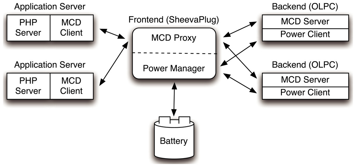
Figure 6: To explicitly control the mapping of keys to servers, we interpose always-active request proxies between memcached clients and servers.
The proxies are able to monitor per-key hit rates and migrate similarly popular objects to the same nodes.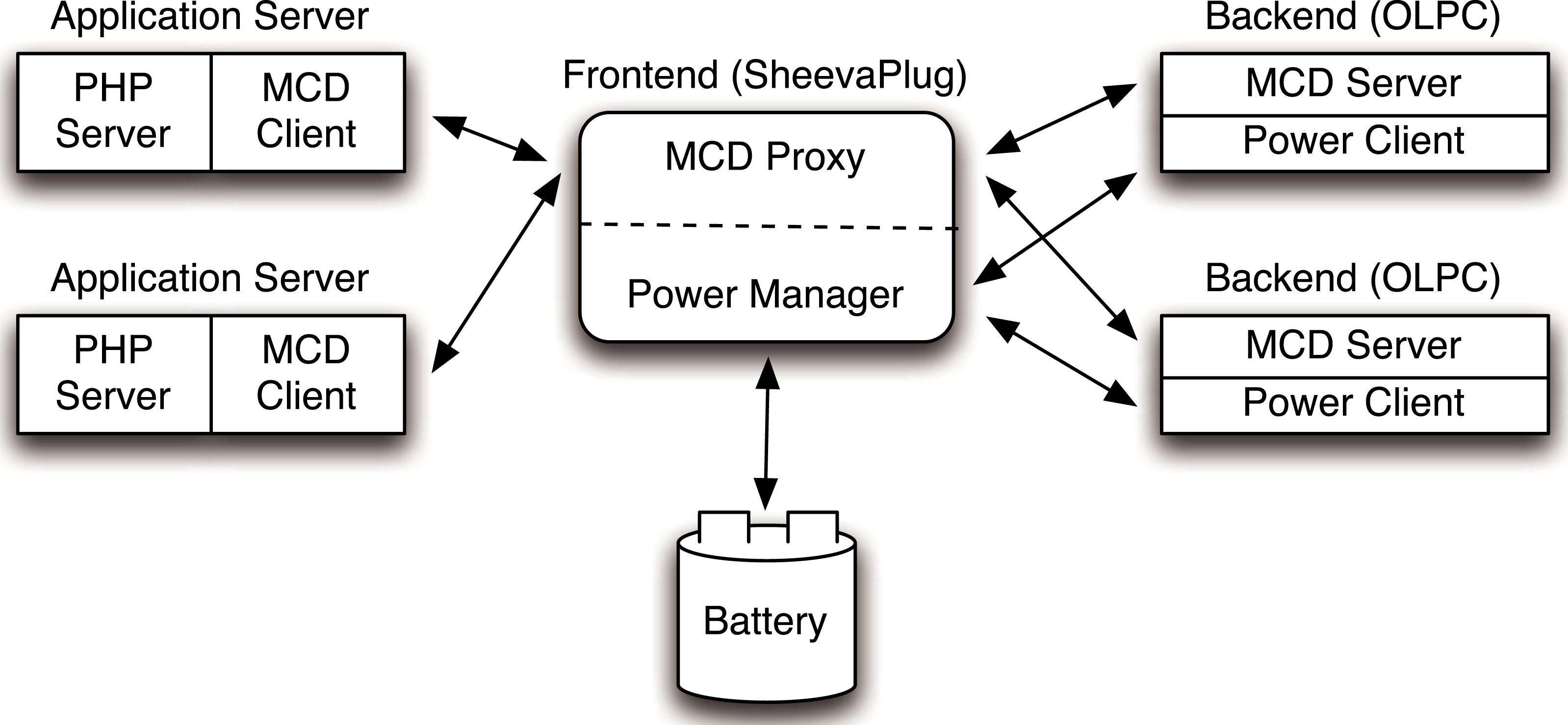
Synchronous policy
The migration-enabled activation policy, described above, approaches the optimal policy for maximizing the cache’s hit rate, since ranking servers and mapping objects to them according to popularity rank makes the distributed cache operate like a centralized cache that simply stores the most popular objects regardless of the cache’s size. We define optimal as the hit rate for a centralized cache of the same size as the distributed Memcached instance under the same workload. However, the policy is unfair for servers that store similarly popular objects, since these servers should have equal rankings. The activation policy is forced to arbitrarily choose a subset of these equally ranked servers to deactivate. In this case, a synchronous policy is significantly more fair and results in nearly the same hit rate as the optimal activation policy. To see why, consider the simple 4-node memcached cluster in Fig. 7 with enough available power to currently activate half the cluster. There is enough power to support either (i) our activation policy with migration that keeps two nodes continuously active or (ii) a synchronous policy that keeps four nodes active half the time but synchronously blinks them between the active and inactive state.
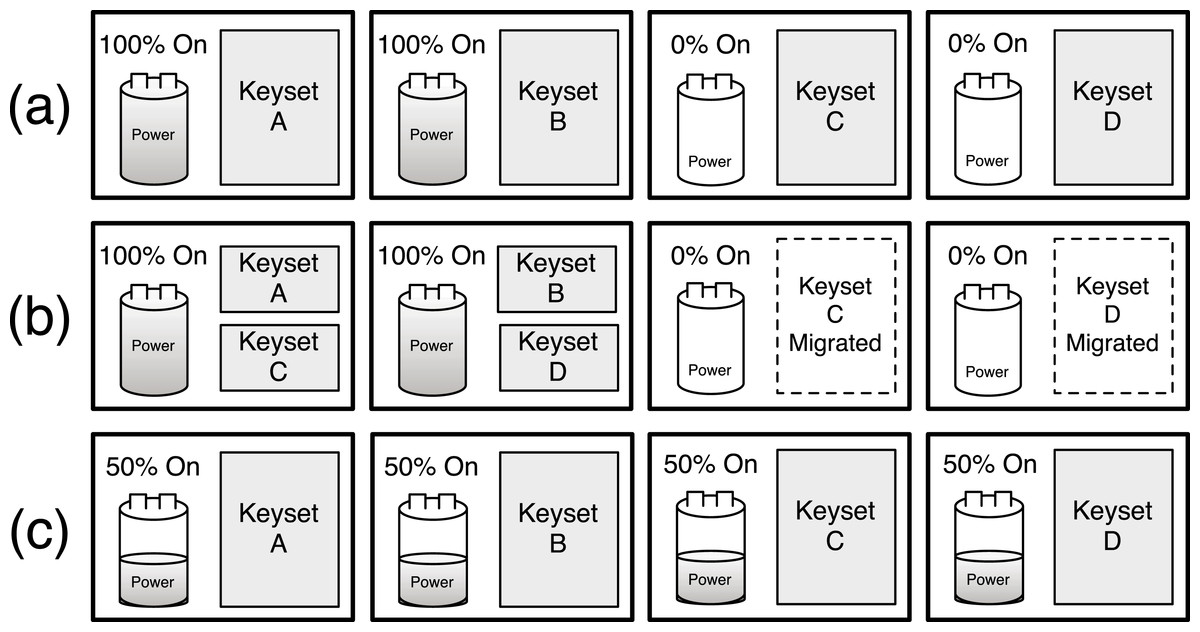
Figure 7: Graphical depiction of a static/dynamic activation blinking policy (A), an activation blinking policy with key migration (B), and a synchronous blinking policy (C).
For now we assume that all objects are equally popular, and compare the expected hit rate and standard deviation of average latency across objects for both policies, assuming a full cache can store all objects at full power on the 4 nodes. For the activation policy, the hit rate is 50%, since it keeps two servers active and these servers store 50% of the objects. Since all objects are equally popular, migration does not significantly change the results. In this case, the standard deviation is 47.5 ms, assuming an estimate of 5 ms to access the cache and 100 ms to regenerate the object from persistent storage. For a synchronous policy, the hit rate is also 50%, since all 4 nodes are active half the time and these nodes store 100% of the objects. However, the synchronous policy has a standard deviation of 0 ms, since all objects have a 50% hit probability, if the access occurs when a node is active, and a 50% miss probability, if the access occurs when a node is inactive. Rather than half the objects having a 5 ms average latency and half having a 100 ms average latency, as with activation, a synchronous policy ensures an average latency of 52.5 ms across all objects.
Note that the synchronous policy is ideal for a normal memcached cluster with a mapping function that randomly maps keys to servers, since the aggregate popularity of objects on each server will always be roughly equal. Further, unlike an activation policy that uses the dynamic mapping function, the synchronous policy does not incur invalidation penalties and is not arbitrarily unfair to keys on lower-ranked servers.
Load-proportional policy
A synchronous policy has the same hit rate as an activation policy when keys have the same popularity, but is significantly more fair. However, an activation policy with migration is capable of a significantly higher hit rate for highly skewed popularity distributions. A proportional policy combines the advantages of both approaches for Zipf-like distributions, where a few key values are highly popular but there is a heavy, but significant, tail of similarly unpopular key values. As with our activation policy, a proportional policy ranks servers and uses a proxy to monitor object popularity and migrate objects to servers in rank order. However, the policy distributes the available power to servers in the same proportion as the aggregate popularity of their keys.
For example, assume that in our 4 server cluster after key migration the percentage of total hits that go to the first server is 70%, the second server is 12%, the third server is 10%, and the fourth server is 8%. If there is currently 100 W of available power then the first server ideally receives 70 W, the second server 12 W, the third server 10 W, and the fourth server 8 W. These power levels then translate directly to active durations over each interval T. In practice, if the first server’s maximum power is 50 W, then it will be active the entire interval, since its maximum power is 70 W. The extra 20 W is distributed to the remaining servers proportionally. If all servers have a maximum power of 50 W, the first server receives 50 W, the second server receives 20 W, i.e., 40% of the remaining 50 W, the third server receives 16.7 W, and the fourth server receives 13.3 W. These power levels translate into the following active durations for a 60 s blink interval: 60 s, 24 s, 20 s, and 16 s, respectively.
| Metric | Workload | Best policy |
|---|---|---|
| Hit Rate | Uniform | Synchronous |
| Hit Rate | Zipf | Activation (Migration) |
| Fairness | Uniform/Zipf | Synchronous |
| Fairness + Hit Rate | Zipf | Load-proportional |
The hit rate from a proportional policy is only slightly worse than the hit rate from the optimal activation policy. In this example, we expect the hit rate from an activation policy to be 85% of the maximum hit rate from a fully powered cluster, while we expect the hit rate from a proportional policy to be 80.2%. However, the policy is more fair to the 3 servers—12%, 10%, and 8%—with similar popularities, since each server receives a similar total active duration. The Zipf distribution for a large memcached cluster has similar attributes. A few servers store highly popular objects and will be active nearly 100% of the time, while a large majority of the servers will store equally unpopular objects and blink in proportion to their overall unpopularity.
Summary
Table 4 provides a summary of the best policy for each performance metric and workload combination. In essence, an activation policy with key migration will always have the highest hit rate. However, for distributions with equally popular objects, the synchronous policy achieves a similar hit rate and is more fair. A load-proportional policy combines the best attributes of both for Zipf-like distributions, which include a few popular objects but many similarly unpopular objects. We evaluate these design alternatives in ‘Evaluation.’
GreenCache: Blinking Multimedia Cache
In the previous section we described how a stateless in-memory cache server can leverage the blinking abstraction to perform well on intermittent power. In this section, we study the characteristics of a distributed multimedia cache, which serves videos requested by clients, either by fetching them from the cache or retrieving them from backend servers. We assume the cache is write-through in that it stores cached videos on disk. A distributed multimedia cache is different than Memcached in many ways—(a) it is not a key-value storage system and, unlike Memcached, it streams data to multimedia players, (b) it stores data on persistent storage and its data size is often much larger than that of Memcached, and (c) like any streaming server it can push data in advance to multimedia players to minimize buffering time and enhance viewers’ experience. In our analysis, we use traces of YouTube traffic as our data source, since YouTube is one of the most popular user-generated video content site and Google deploys 1,000s of servers to serve YouTube requests made by users all around the world.
Multimedia cache overview
Multimedia caches are widely used to reduce backhaul bandwidth usage and improve viewers’ experience by reducing buffering time or access latency. Apart from traditional multimedia servers, network operators have also started deploying multimedia caches at cellular towers to cater for the growing demand of multimedia content from smartphone users. Traditionally, network operators have deployed caches only at centralized locations, such as operator peering points, in part, for both simplicity and ease of management (Xu et al., 2011). However, researchers and startups have recently recognized the benefit of placing caches closer to edge (Xu et al., 2011; Stoke Solutions, 2011). Co-locating server caches closer to cell towers reduces both access latency, by eliminating the need to route requests for cached data through a distant peering point, and backhaul bandwidth usage from the cell tower to the peering point. Caches co-located with cell towers primarily target multimedia data, since it consumes the largest fraction of bandwidth and is latency-sensitive.
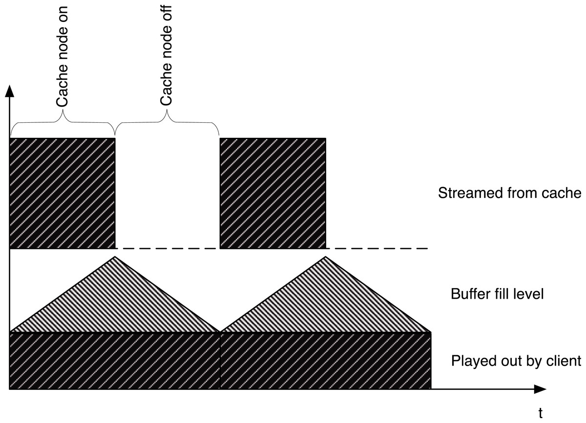
Figure 8: The top part of the figure shows a potential streaming schedule for a blinking node while the bottom half shows the smooth play out with is achieved with the aid of a client-side buffer.
We study the design of GreenCache in the context of such a distributed multimedia cache for cellular towers. Many of these cellular towers, especially in developing countries, are located in remote areas without reliable access to power. As a result, renewable energy sources have been proposed to power these cellular towers (Guay, 2012; Balshe, 2011). To handle intermittency in the power supply, we assume a cache architecture that comprises of a number of low-power servers, since a single large cache is not energy-proportional, and, thus, not well-suited to operating off intermittent renewable energy sources. The advantage of a distributed multimedia cache is that it allows the cache size to scale up and down based on available power. However, it introduces a new complication: if servers are inactive due to power shortages by renewables then the data cached on them becomes unavailable. If data resides on an inactive server, the client must either wait until the server is active, e.g., there is enough power, or retrieve the already cached data again from the origin server.
In this case, the blinking abstraction enables the cache to provide service, albeit at degraded performance, during shortfall periods. In essence, blinking provides a cache with new options in its design space. Rather than having a small cache composed of the number of always-on servers the available power can sustain, blinking provides the option of having a much larger cache composed of servers that are active for only a fraction of time each blink interval, e.g., active for 10 s during each minute interval. The use of blinking raises new challenges in multimedia cache design. The main challenge is to ensure smooth uninterrupted video playback even while blinking. Doing so implies that caches have to stream additional data during their active periods to compensate for lack of network streaming during sleep periods. Further, end-clients will need to employ additional client-side buffers and might see higher startup latencies.
Since multimedia applications are very sensitive to fluctuation in network bandwidth that might cause delayed data delivery at the client, most applications prefer that video players employ a buffer to smooth out such fluctuations and provide an uninterrupted, error free play out of the data. This buffer, which already exists for most multimedia applications on the client side, integrates well into the blinking approach since it also allows the cache to bridge outage times in individual cache servers, as shown in Fig. 8. A blinking cache will stream additional chunks when active, which are buffered at the client. As shown in this figure, the player is then able to play the video smoothly and masks interruptions from the viewer as long as it gets the next chunk of data before the previous chunk has finished playing.
Finally, in a typical cell tower or 3G/4G/WiMAX scenario the downstream bandwidth (∼30–40 Mbps) is much less than the bandwidth a cache server can provide, which is generally limited by its network card and disk I/O. So, the cache server can potentially reduce its energy consumption by sending data at its full capacity for a fraction of a time interval (usually few seconds) and going to a low-power state for the remaining period of the time interval, as shown in Fig. 8. In essence, the server could employ the blinking abstraction to reduce its energy footprint while still satisfying the downstream bandwidth requirement of the cell tower or WiMAX station. Moreover, blinking facilitates a cache to employ more servers than it can keep active with the available power, and thus provides an opportunity to reduce server load and bandwidth usage.
The primary drawback of a blinking cache is that it stalls a request if the requested video is not currently available on an active server. If a client requests a video that is present on an inactive server, the cache can either get the video from the back-end server or the client pauses play out until the inactive server becomes active. While getting the video from the back-end server, instead of waiting for the inactive server to become active, reduces the buffering time, it increases the bandwidth cost. As we describe later in this section, GreenCache uses a low-power always-on proxy and staggered load-proportional blinking policy to reduce buffering time while sending requests to back-end servers only if data is not available in the cache.
YouTube trace analysis
To inform the design of GreenCache based on the characteristics of multimedia traffic and viewer behavior, we analyze a network trace that was obtained by monitoring YouTube traffic entering and leaving a campus network at the University of Connecticut. The network trace is collected with the aid of a monitoring device consisting of PC with a Data Acquisition and Generation (DAG) card (Endace, 2011), which can capture Ethernet frames. The device is located at a campus network gateway, which allows it to capture all traffic to and from the campus network. It was configured to capture a fixed length header of all HTTP packets going to and coming from the YouTube domain. The monitoring period for this trace was 72 h. This trace contains a total of 105,339 requests for YouTube videos out of which ∼80% of the video requests are single requests which leaves about 20% of the multiple requests to take advantage of caching of the requested videos. We would like to point out that a similar caching potential (24% in this case) has been reported in a more global study of 3G networks traffic analysis by Erman et al. (2011).
Figure 9 shows the popularity distribution of the 100 most popular videos, which is obtained based on the user requests recorded in the trace. This figure only shows the 100 most popular videos since the trace contains many videos with a very low popularity (<10 requests) and we wanted to depict the distribution of the most popular videos in more detail. The data obtained from the analysis of the trace shows that, despite the very long tail popularity distribution, caching can have an impact on the performance of such a video distribution system.
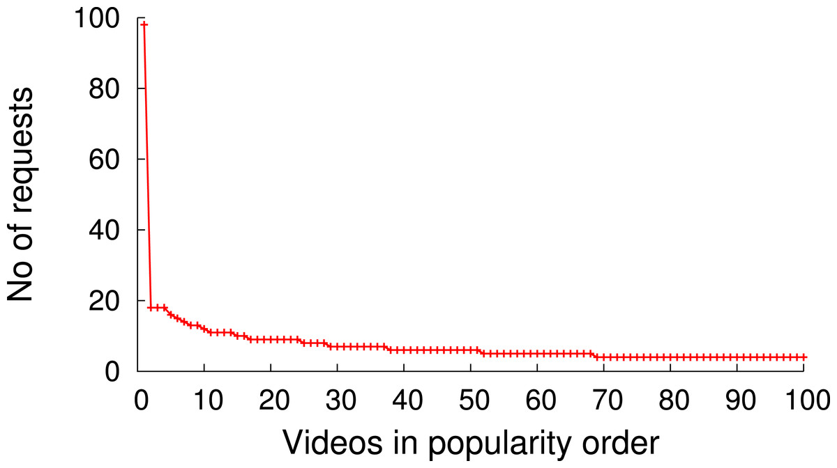
Figure 9: Video popularity (100 out of 105,339).
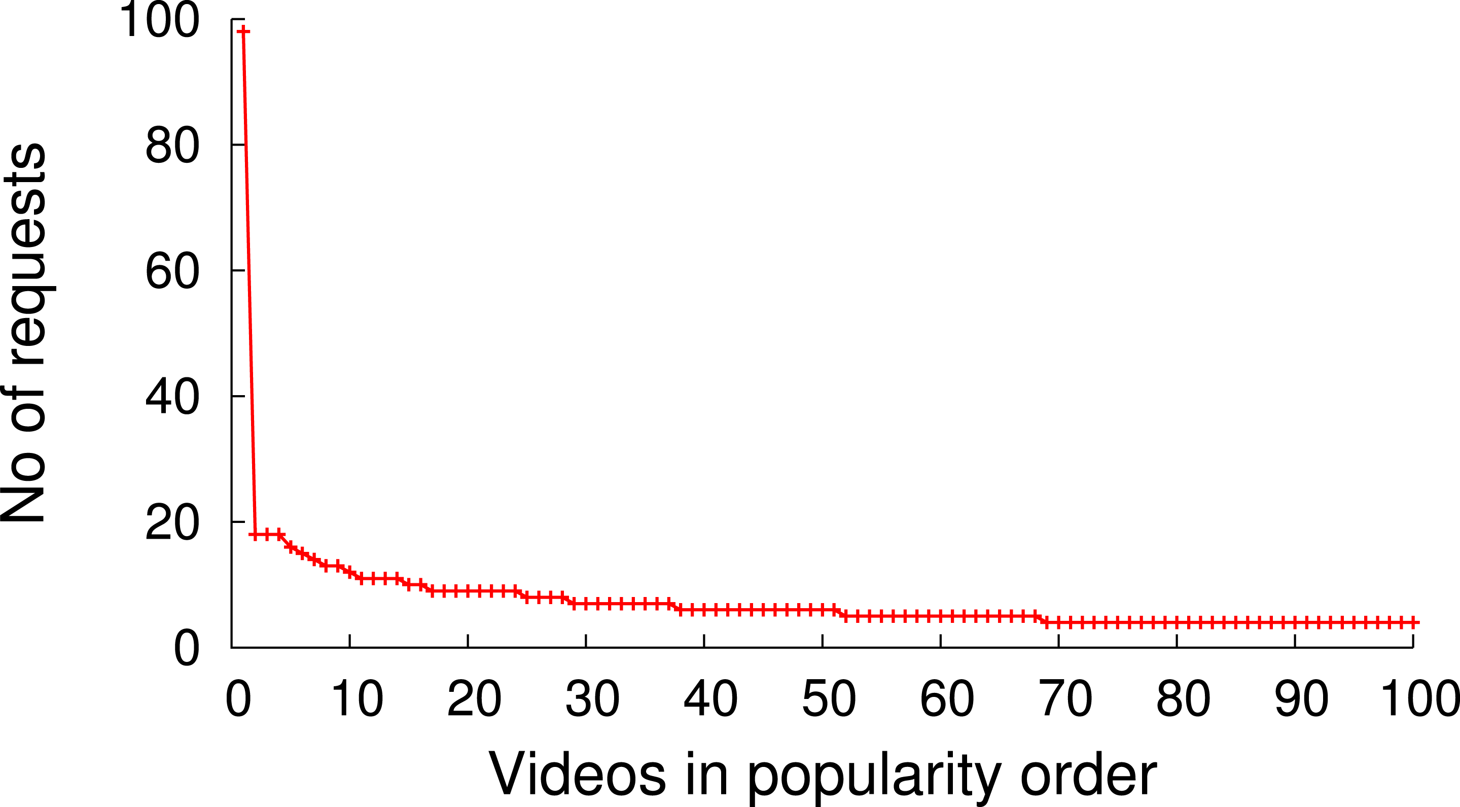
In earlier work (Khemmarart et al., 2011), we have shown that, not only caching but also the prefetching of prefixes of videos that are shown on the related video list of a YouTube video page can improve the viewers experience of watching videos. Further analysis of the trace revealed that 47,986 request out of the 105,339 had the tag related_video (∼45%), which indicates that these videos have been chosen by viewers from the related video list that is shown on each YouTube video’s web page. In addition to identifying videos that are selected from the related list, we also determine the position on the related list the video was selected from and show the result in Fig. 10A. It shows that users tend to request from the top 10 videos shown on the related list of a video, which accounts for 80% of the related video requests in the trace. This data shows that, prefetching the prefixes of the top 10 videos shown on the related list of a currently watched video can significantly increase viewer’s experience, since the initial part can be streamed immediately from a location close to the client. Based on these results, we decided to evaluate a blinking multimedia cache that performs both, traditional caching, and prefix prefetching for the top 10 videos on the related video list.
We also analyze the trace to investigate if viewers switch to a new video before they completely finish watching the current video. In order to analyze this behaviour, we look into the timestamps of a user requesting two consecutive videos. We calculate the difference of these timestamps and compare it with the total length of the first video requested to determine if the user has switched between videos before the previous video is completely viewed.
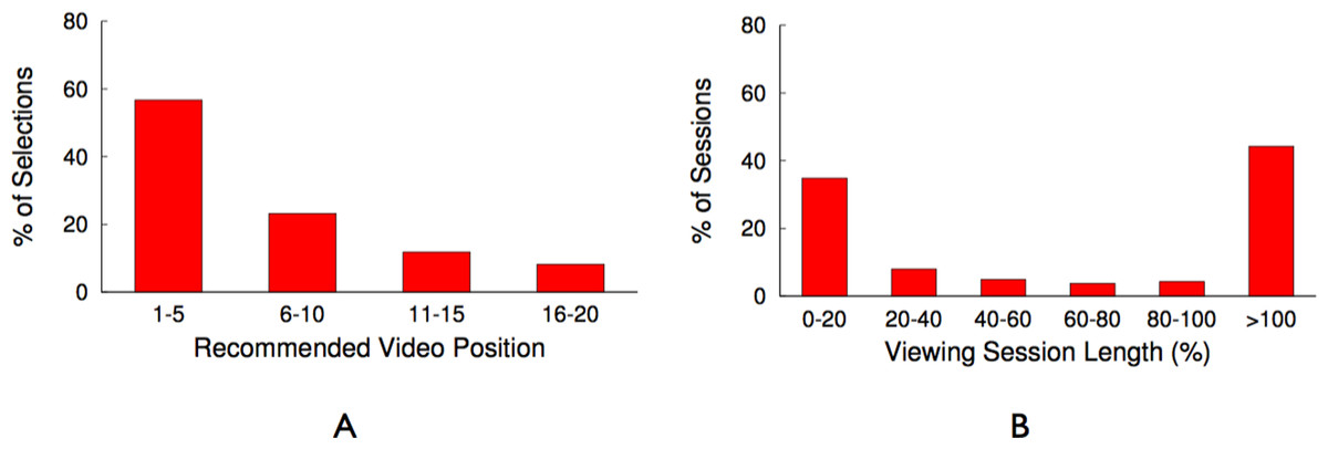
Figure 10: YouTube trace related videos and switch time analysis.
(A) Related video position analysis. (B) Video switching time analysis.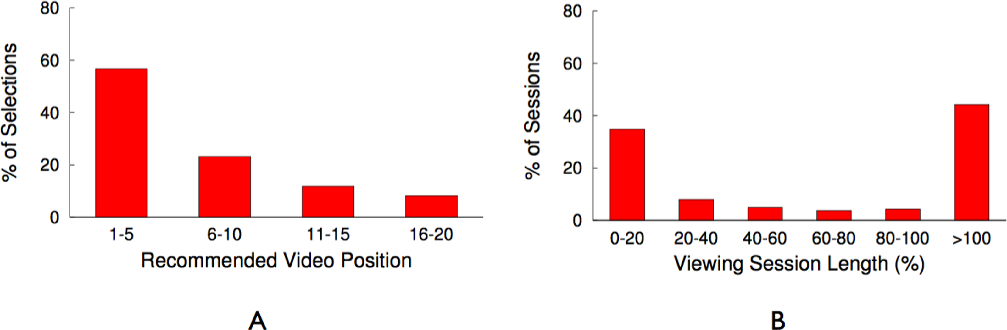
Figure 10B shows the number of occurrences (in percent out of the total number of videos watched) a video is watched for x% of its total length. This result shows that only in 45% of the cases videos are watched completely (also this number is similar to the global study performed by Erman et al. (2011)). In all other cases only part of the video is watched, with the majority of these cases (∼40%) falling in the 0–20% viewing session length. This result let us to the decision to divide a video into equal-sized chunks, which allows for the storage of different chunks that belong to a single video on different nodes of the cache cluster. In ‘Minimizing bandwidth cost,’ we describe how the chunk size is determined and how chunking a video can reduce the uplink bandwidth usage if used on a blinking multimedia cache cluster.
GreenCache design
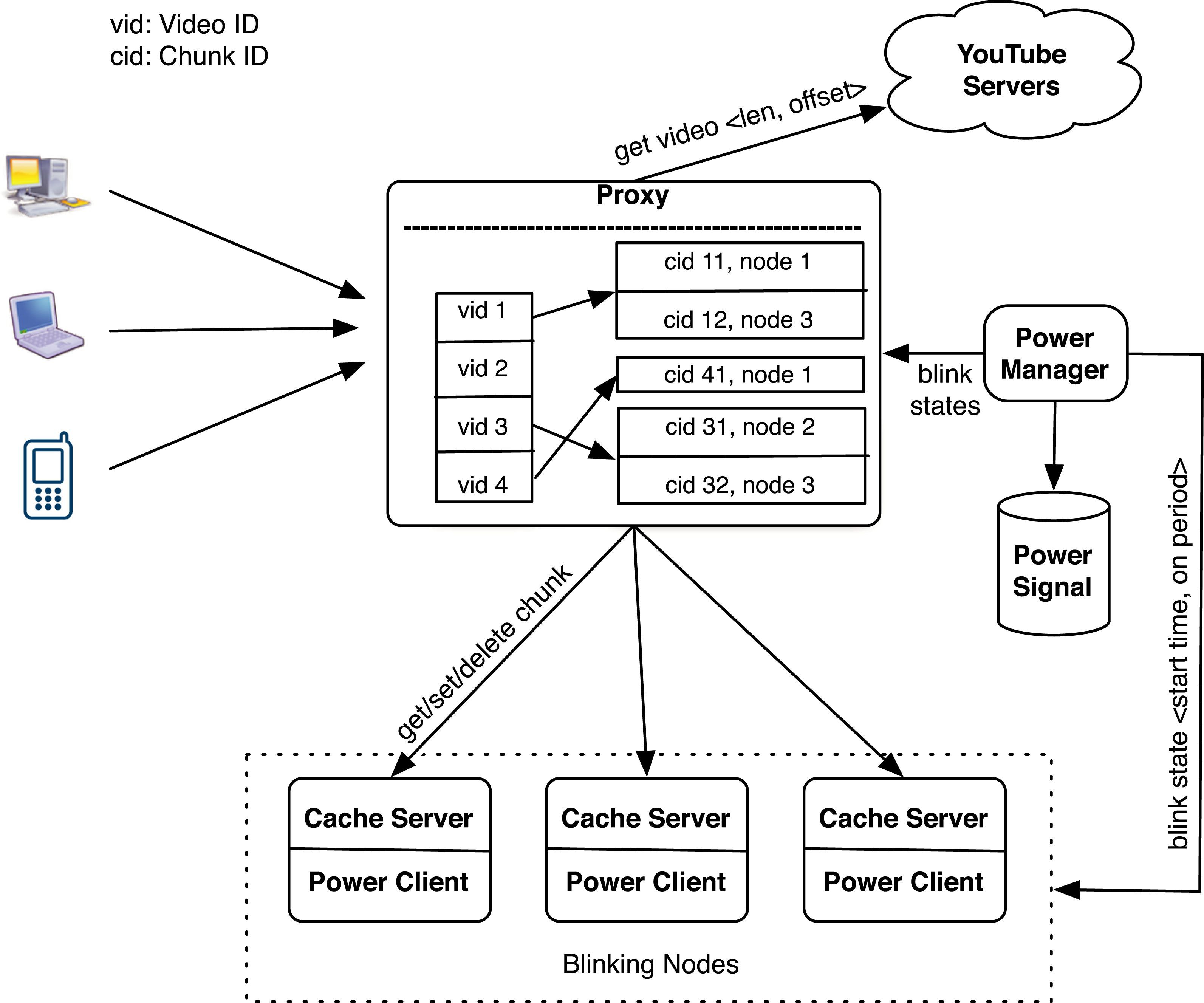
Figure 11 depicts GreenCache’s architecture, which consists of a proxy and several cache servers. The proxy maintains a video → chunk mapping and a chunk → node mapping, while also controlling chunk server placement and eviction. Clients, e.g., web browsers, connect to video servers through the proxy, which fetches the requisite data from one or more of its cache servers, if the data is resident in the cache. If the data is not resident, the proxy forwards the request to the host, i.e., backend server. The proxy stores metadata to access the cache in its own memory, while video chunks reside on stable storage on each cache server.
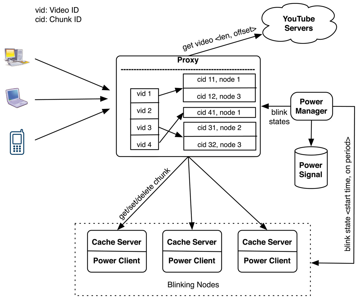
Figure 11: GreenCache architecture.
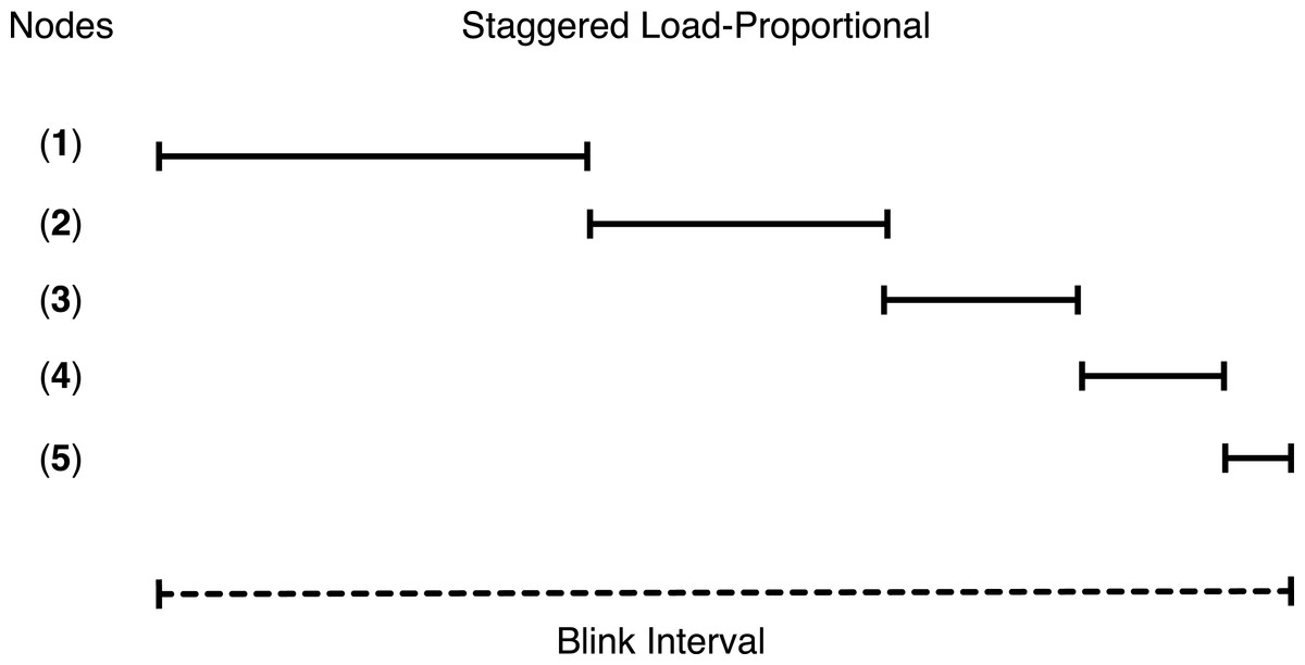
Figure 12: Staggered load-proportional blinking.
Similar to BlinkCache, GreenCache also includes a power manager, that monitors available power and energy stored in a battery using hardware sensors, e.g., a voltage logger and current transducer. The power manager implements various blinking policies to control nodes’ active and inactive intervals to match the cache’s power usage to the available power. The power manager communicates with a power client running on each cache server to set the start time and active period every blink interval. The power client activates the node at the start time and deactivates the node after the active period every blink interval, and thus controls node-level power usage by transitioning the node between active and inactive states.
As discussed earlier, the primary objective of a multimedia cache is to reduce buffering (or pause) time at clients and the bandwidth usage between the cache and origin servers. Next, we describe GreenCache’s techniques to both reduce bandwidth usage to the backend origin servers, while also minimizing buffering (or pause) time at the client.
Minimizing bandwidth cost
As Fig. 9 indicates, all videos are not equally popular. Instead, a small number of videos exhibit a significantly higher popularity than others. Similar to other multimedia caches, GreenCache has limited storage capacity, requiring it to evict older videos to cache new videos. An eviction strategy that minimizes the bandwidth usage each interval will evict the least popular videos during the next interval. However, such a strategy is only possible if the cache knows the popularity of each video in advance. To approximate a video’s future popularity, GreenCache maintains each video’s popularity as an exponentially-weighted moving average of a video’s accesses, updated every blink interval. The cache then evicts the least popular videos if it requires space to store new videos.
As shown in Fig. 10B, most videos are not watched completely most of the time. In fact, the figure shows that users of YouTube watch less than 45% of the videos to completion. In addition, users might watch the last half of a popular video less often than the first half of an unpopular video. To account for discrepancies in the popularity of different segments of a video, GreenCache divides a video into multiple chunks, where each chunk’s playtime is equal in length to the blink interval. Similar to entire videos, GreenCache tracks chunk-level popularity as an exponentially weighted moving average of a chunk’s accesses. Formally, we can express the popularity of the ith chunk after the tth interval as: (1)
Ait represents the total number of accesses of the ith chunk in the tth interval, and α is a configurable parameter that weights the impact of past accesses. Further, GreenCache manages videos at the chunk level, and evicts least popular chunks, from potentially different videos, to store a new chunk. As a result, GreenCache does not need to request chunks from the backend origin servers if the chunk is cached at one or more cache servers.
Reducing buffering time
As discussed earlier, blinking increases buffering time up to a blink interval, if the requested chunk is not present on an active server. The proxy could mask the buffering time from a client if the client receives a chunk before it has finished playing the previous chunk. Assuming sufficient energy and bandwidth, the proxy can get a cached chunk from a cache server within a blink interval, since all servers become active for a period during each blink interval. As a result, a user will not experience pauses or buffering while watching a video in sequence, since the proxy has enough time to send subsequent chunks (after the first chunk) either from the cache or the origin server before the previous chunk finishes playing, e.g., within a blink interval. However, the initial buffering time for the first chunk could be as long as an entire blink interval, since a request could arrive just after the cache server storing the first chunk becomes inactive. Thus, to reduce the initial buffering time for a video, the proxy replicates the first chunk of cached videos on all cache servers. However, replication alone does not reduce the buffering time if all servers blink synchronously, i.e., become active at the same time every blink interval. As a result, as discussed next, GreenCache employs a staggered load-proportional blinking policy to maximize the probability of at least one cache server being active at any power level.
Staggered load-proportional blinking
As discussed above, we replicate the first chunk of each cached video on all cache servers in order to reduce initial buffering time. To minimize the overlap in node active intervals and maximize the probability of at least one active node at all power levels, GreenCache staggers start times of all nodes across each blink interval. Thus, every blink interval, e.g., 60 s, each server is active for a different period of time, as well as a different duration (discussed below). At any instant, a different set of servers (and their cached data) is available for clients. Since at low power the proxy might not be able to buffer all subsequent chunks from blinking nodes, clients might face delays or buffering while watching videos (after initially starting them).
To reduce the intermediate buffering for popular videos, GreenCache also groups popular chunks together and assigns more power to nodes storing popular chunks than nodes storing unpopular chunks. Thus, nodes storing popular chunks are active for a longer duration each blink interval. GreenCache ranks all servers from 1…N, with 1 being the most popular and N being the least popular node. The proxy monitors chunk popularity and migrates chunks to servers in rank order. Furthermore, the proxy distributes the available power to nodes in proportion to the aggregate popularity of their chunks. Formally, active period for the ith node, assuming negligible power for inactive state, could be expressed as (2)
BI represents the length of a blink interval, Popularityi represents the aggregate popularity of all chunks mapped on the ith node, P denotes the available power, and MP is the maximum power required by an active node. Additionally, start times of nodes are staggered in a way that minimizes the unavailability of first chunks, i.e., minimizes the period when none of the nodes are active, every blink interval. Figure 12 depicts an example of staggered load-proportional blinking for five nodes. Note that since the staggered load-proportional policy assigns active intervals in proportion to servers’ popularity, it does not create an unbalanced load on the cache servers.
Prefetching recommended videos
Most popular video sites display a recommended list of videos to users. For instance, YouTube recommends a list of twenty videos which generally depends on the current video being watched, the user’s location, and other factors including past viewing history. The trace analysis of YouTube videos, as discussed above, indicates that users tend to select the next video from recommended videos ∼45% of the time. In addition, a user selects a video at the top more often than a video further down in the recommended list. In fact, Fig. 10A shows that nearly 55% of the time a user selects the next video from top five videos in the recommended list. To further reduce initial buffering time the proxy prefetches the first chunk of top five videos in the recommended list, if these chunks are not already present in the cache. The proxy fetches subsequent chunks of the video when the user requests the video next.
Implementation
We use the Blink’s hardware and software prototype from ‘Blink Prototype’ to experiment with BlinkCache and GreenCache. We use the low-power server cluster of XO motherboards for BlinkCache, and that of Mac minis for GreenCache.
BlinkCache implementation
We run an unmodified memcached server and an instance of Blink’s power client on each BlinkCache node. We also wrote a memcached client workload generator to issue key requests at a configurable but steady rate according to either a Zipf popularity distribution, parameterized by α, or a uniform popularity distribution. As in a typical application, the workload generator fetches any data not resident in the cache from a MySQL database and places it in the cache. Since we assume the MySQL server provides always-available persistent storage, it runs off the power grid and not variable power. We modify magent, a publicly available memcached proxy (http://code.google.com/p/memagent/), to implement the design alternatives in the previous section, including table-based key mapping and popularity-based key migration. Our modifications are not complex: we added or changed only 300 lines of code to implement all of the BlinkCache design variants from ‘Blink Prototype.’ Since all requests pass through the proxy, it is able to monitor key popularity. The proxy controls blinking by interacting with Blink’s power manager, which in our setup runs on the same node, to monitor the available power and battery level and set per-node blinking patterns. We also use the proxy for experiments with memcached’s default hash-based key mappings, rather than modifying the memcached client. Since our always-on proxy is also subject to intermittent power constraints, we run it on a low-power (5 W) embedded SheevaPlug with a 1.2 GHz ARM CPU and 512 MB of memory.
GreenCache implementation
As discussed in ‘GreenCache: Blinking Multimedia Cache,’ we study the GreenCache’s design in the context of a cellular tower powered by solar and wind energy. In our prototype we use a WiMAX base station to emulate the cellular tower. To analyze the blinking performance of GreenCache, we implement a GreenCache prototype in Java, including a proxy (∼1,500 LOC), cache server (∼500 LOC), power manager (∼200 LOC), and power client (∼150 LOC). Mobile clients connect to the Internet through a wireless base station, such as a cell tower or WiMAX base station, which is configured to route all multimedia requests to the proxy. While the power manager and proxy are functionally separate and communicate via well-defined APIs, our prototype run both modules on the same node. Our prototype does not require any modification in the base station or mobile clients. Both cache server and power client run together on each blinking node.
Our prototype includes a full implementation of GreenCache, including the staggered load-proportional blinking policy, load-proportional chunk layout, prefetching, video chunking, chunk eviction and chunk migration. The proxy uses a Java Hashtable to map videos to chunks and their locations, e.g., via their IP address, and maintains their status, e.g., present or evicted. Since our prototype has a modular implementation, we are able to experiment with other blinking policies and chunk layouts. We implement the activation and proportional policies similar to the memcached application as described in ‘BlinkCache: Blinking Memcached’ and compare with GreenCache’s staggered load-proportional policy. We also implement a randomized chunk layout and the Least Recently Used (LRU) cache eviction policy to compare with the proposed load-proportional layout and popularity based eviction policy, respectively.
As discussed in ‘Blink Prototype,’ we use a cluster of ten Mac minis for GreenCache. We use one Mac mini to run the proxy and power manager, whereas we run a cache server and power client on other Mac minis. The proxy connects to a WiMAX base station (NEC Rel.1 802.16eBS) through the switch. We use a Linux laptop with a Teletonika USB WiMAX modem to run as a client. We also use a separate server to emulate multiple WiMAX clients. Our emulator limits the wireless bandwidth, in the same way as observed by the WiMAX card, and plays the YouTube trace described below. The WiMAX base station is operational and located on the roof of a tall building on the UMass campus. However, the station is currently dedicated for research purposes and is not open to the general public. Since GreenCache requires one node, running the proxy and power manager, the switch, and WiMAX base station to be active all the time, its minimum power consumption is 46 W, or 17% of its maximum power consumption.
To experiment with a wide range of video traffic, we wrote a mobile client emulator in Java, which replays YouTube traces. For each video request in the trace file, the emulator creates a new thread at the specified time to play the video as per the specified duration. In addition, the emulator also generates synthetic video requests based on various configurable settings, such as available bandwidth, popularity distribution of videos, e.g., a Zipf parameter, viewing length distribution, and recommended list distribution.
Blink emulator
To study how the BlinkCache and GreenCache design scales with the cluster size we write an emulator that emulates a server cluster. The emulator takes the number of servers, servers’ parameters (e.g., RAM, IP Address, Port), network bandwidth, and the application name as input parameters, and starts as many processes as the number of servers. Each process emulates a node in the cluster, and applications running on that node are started in separate threads in the process. For example, a blinking node in BlinkCache is emulated by a process with two threads—one thread runs a power client while the other runs a memcached server. The power manager takes the power trace from our field deployment and scales up the trace to bring the average power at 50% of the power necessary to run all nodes concurrently. To emulate blinking of a node the power client sends the process to the sleep state and active state as directed by the power manager.
We run our Blink emulator on a Mac mini running Linux kernel 2.6.38 with 2.4 GHz Intel Core 2 Duo processor and 8 GB of RAM. The emulator starts up to 1,000 processes to emulate 1,000 blinking nodes. We use benchmark results from our low-power server cluster to set application-level configuration parameters, such as request rate, access latency, transition latency, power consumption, zipf parameter, servers to proxy ratio etc., for applications running on the Blink emulator. As in our real cluster all modules and applications communicate over TCP/IP. Further, to run a memcached server in a thread, rather than in a process, we write a small memcached emulator that emulates basic operations (single-key get and put) of Memcached with similar latencies as observed with a real memcached server in our evaluation (‘Evaluation’).
Power signal
We program our power supplies to replay solar and wind traces from our field deployment of solar panels and wind turbines. We also experiment with both multiple steady and oscillating power levels as a percentage, where 0% oscillation holds power steady throughout the experiment and N% oscillation varies power between (45 + 0.45N)% and (45 − 0.45N)% every five minutes. We combine traces from our solar/wind deployment, and set a minimum power level equal to the power necessary to operate the always-active components. We compress our renewable power signal to execute three days in three hours, and scale the average power to 50% of the cluster’s maximum power.
Evaluation
We evaluate BlinkCache and GreenCache on our small-scale Blink prototype from ‘Blink Prototype’. The purpose of our evaluation is not to maximize the performance of a particular deployment of our applications—memcached and multimedia cache—or improve on the performance of the custom deployments common in industry. Instead, our goal is to explore the effects of churn on the applications caused by power fluctuations for different design alternatives. Our results will differ across platforms according to the specific blink interval, CPU speed, and network latency and bandwidth of the servers and the network. Since our prototype uses low-power CPUs and motherboards, the request latencies we observe in our prototype are not representative of those found in high performance servers.
BlinkCache evaluation
We first use our workload generator to benchmark the performance of each blinking policy for both Zipf-like and uniform popularity distributions at multiple power levels with varying levels of oscillation. We then demonstrate the performance for an example web application—tag clouds in GlassFish—using realistic traces from our energy harvesting deployment that have varying power and oscillation levels. Unless otherwise noted, in our experiments, we use moderate-size objects of 10 KB, Facebook-like Zipf α values of 0.6, and memcached’s consistent hashing mapping function. Each experiment represents a half-hour trace, we configure each memcached server with a 100 MB cache to provide an aggregate cache size of 1 GB, and we use our programmable power supply to drive each power trace. Since each node has only 256 MB of memory, we scale our workloads appropriately for evaluation.
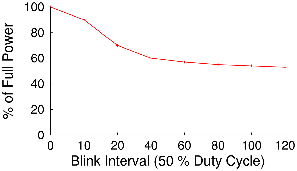
Figure 13: The near 2 s latency to transition into and out of S3 in our prototype discourages blinking intervals shorter than roughly 40 s.
With a 50% duty cycle we expect to operate at 50% full power, but with a blink interval of less than 10 s we operate near 100% full power.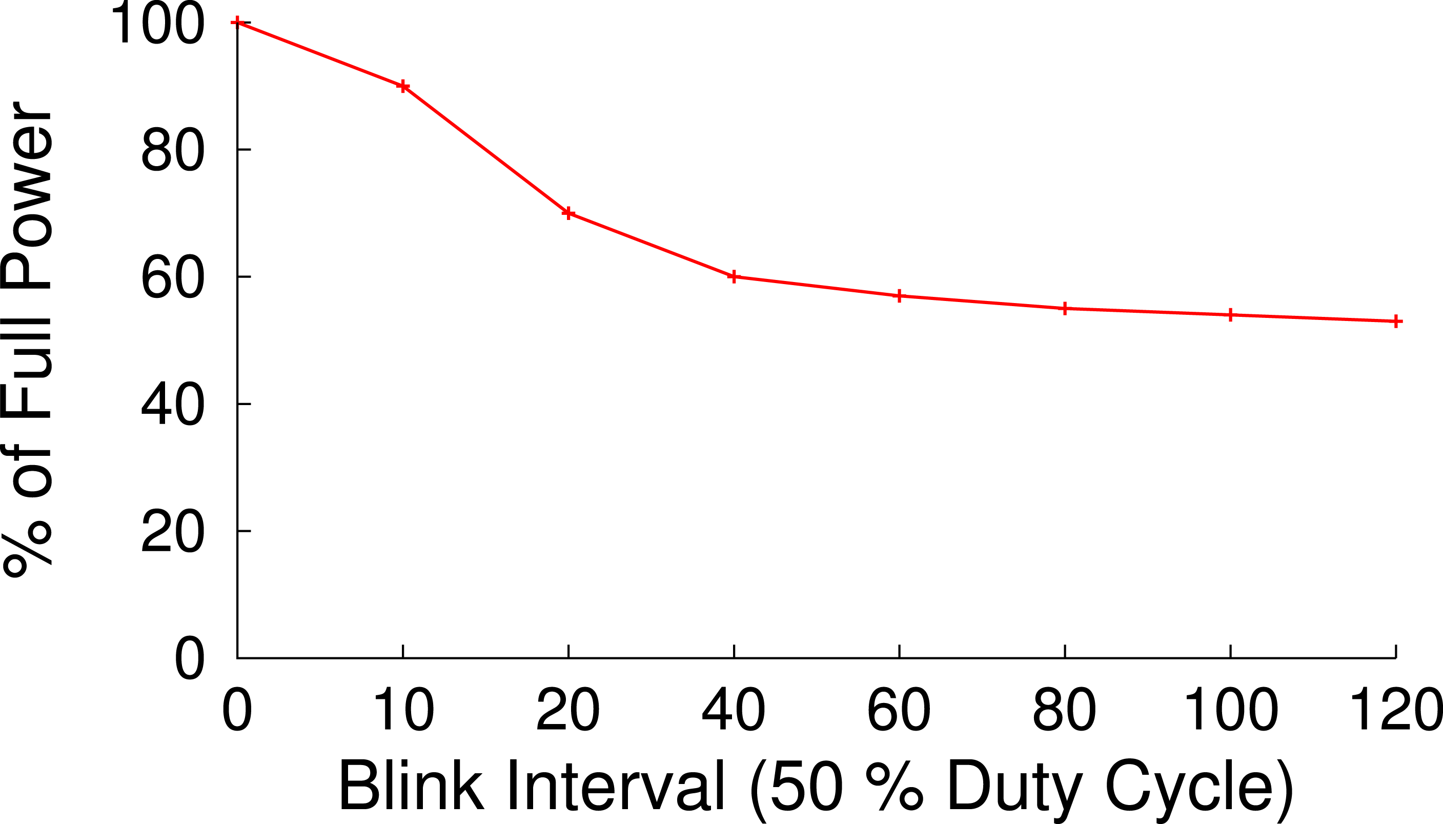
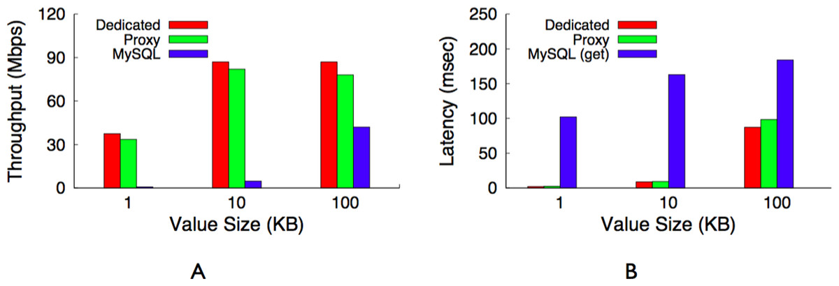
Figure 14: Maximum throughput (A) and latency (B) for a dedicated memcached server, our memcached proxy, and a MySQL server.
Our proxy imposes only a modest overhead compared with a dedicated memcached server. (A) Throughput. (B) Latency.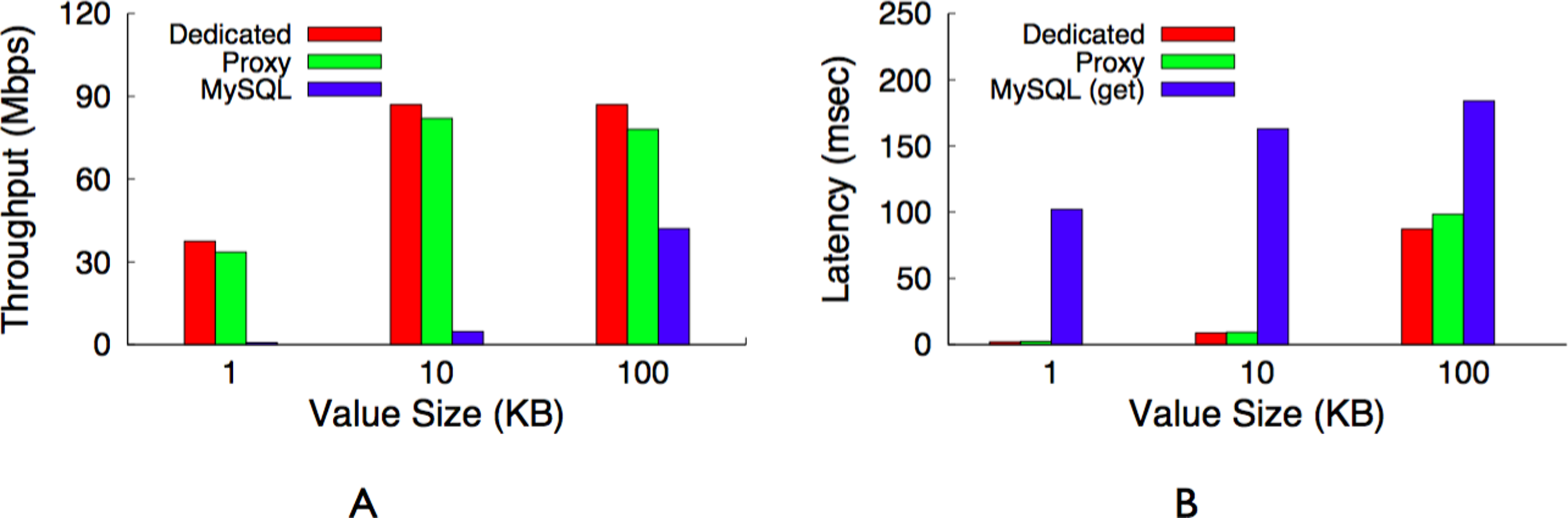
Benchmarks
We measure the maximum power of each node, at 100% CPU and network utilization, in S0 to be 8.6 W and its minimum power in S3 to be 0.2 W. We use these values in the proxy to compute the length of active and inactive periods to cap power consumption at a specific level. We also measure the impact of our node’s near 2 s transition latency for blink intervals T between 10 s and 2 min. Figure 13 shows the results for a duty cycle of 50%. In this case, the blinking interval must be over 40 s before average power over the interval falls below 55% of the node’s maximum power, as we expect. The result shows that on-demand transitions that occur whenever work arrives or departs are not practical in our prototype. Further, even blinking intervals as high as 10 s impose significant power inefficiencies. As a result, we use a blinking interval of 60 s for our experiments. Our 60 s blink interval is due solely to limitations in the Blink prototype. Note that there is an opportunity to significantly reduce blink intervals through both hardware and software optimizations. Since server clusters do not typically leverage ACPI’s S3 state, there has been little incentive to optimize its transition latency.
Next, we determine a baseline workload intensity for memcached, since, for certain request rates and key sizes, the proxy or the switch becomes a bottleneck. In our experiments, we use a steady request rate (1,000 get requests/s) that is less than the maximum request rate possible once the proxy or switch becomes a bottleneck. Note that our results, which focus on hit rates, are a function of the popularity of objects rather than the distribution of request inter-arrival times. Our goal is to evaluate how blinking affects the relative hit rates between the policies, and not the performance limitations of our particular set of low-power components. Figure 14 demonstrates the maximum performance, in terms of total throughput and request latency for different key values sizes, of an unmodified memcached server, our memcached proxy, and a MySQL server. As expected, the memcached server provides an order of magnitude higher throughput and lower request latency than MySQL. Further, our proxy implementation imposes only a modest overhead to both throughput and latency, although the latency impact of proxy-based redirections will be greater on faster CPUs since less relative request time is spent in the OS and network. Our subsequent experiments focus on request hit rates rather than request latencies, since latencies vary significantly across platforms and workloads. Further, the wide disparity in latency between serving a request from memory and serving it from disk would show a larger, and potentially unfair, advantage for a blinking system. Thus, we consider hit rate a better metric than latency for evaluating a blinking memcached instance.
Activation blinking and thrashing
An activation policy for an unmodified version of memcached must choose whether or not to alter the hash-based mapping function as it activates and deactivates servers. For constant power, a dynamic mapping function that always reflects the currently active set of servers should provides the best hit rate, regardless of the popularity distribution, since applications will be able to insert the most popular keys on one of the active servers. Figure 15A demonstrates this point for a workload with a Zipf popularity distribution (α = 0.6), and shows the hit rates for both static and dynamic activation variants at multiple constant power levels. While at high power levels the approaches have similar hit rates, as power level decreases, we see that the static variant incurs a higher penalty under constant power. However, Fig. 15B demonstrates that the opposite is true for highly variable power. The figure reports hit rates for different levels of power oscillation, where the average power for each experiment is 45% of the power necessary to run all nodes concurrently. The x-axis indicates oscillation level as a percentage, such that 0% oscillation holds power steady throughout the experiment and N% oscillation varies power between (45 + 0.45N)% and (45 − 0.45N)% every 5 min.

Figure 15: Hit rate with activation policy under constant and oscillating power for a Zipf popularity distribution.
(A) Constant power. (B) Variable power.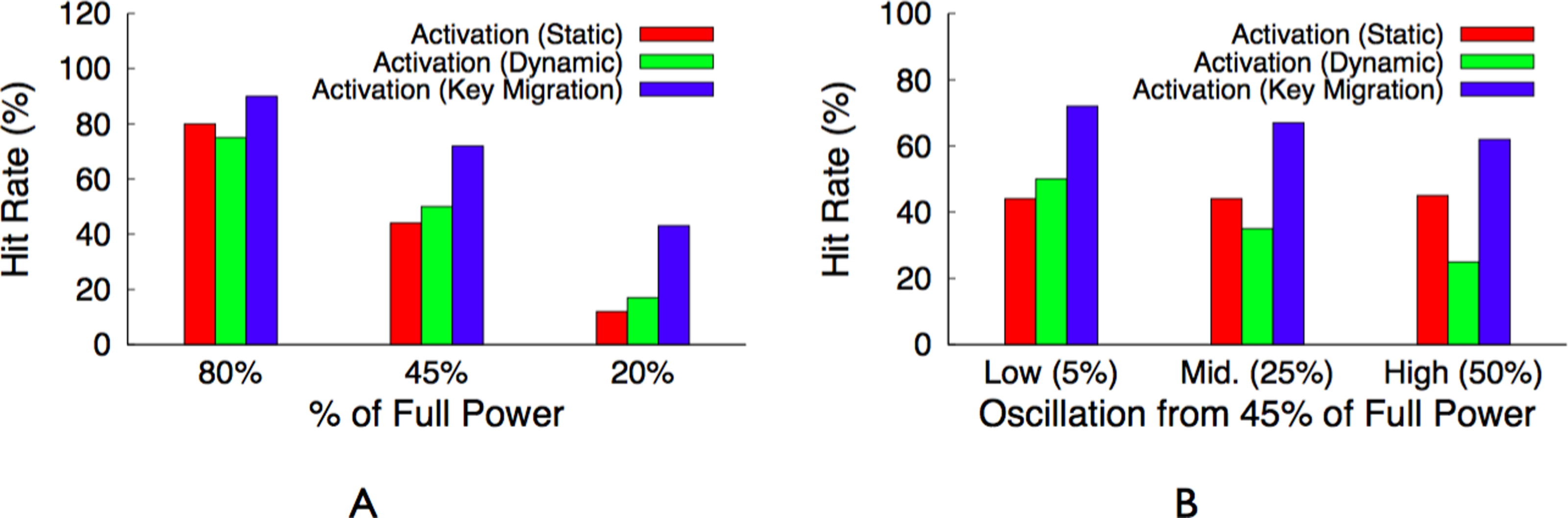
We see that dynamic changes in the active server set of memcached’s hash-based mapping function incur an invalidation penalty. Since the invalidation penalty does not occur when memcached does not change the mapping function, the static variant provides a significantly better hit rate as the oscillations increase. Although not shown here, the difference with the original modulo approach is much greater, since each change flushes nearly the entire cache. The hash-based mapping function forces a choice between performing well under constant power or performing well under variable power. A table-based approach that uses our proxy to explicitly map keys to servers and uses key migration to increase the priority of popular keys performs better in both scenarios. That is, the approach does not incur invalidation penalties under continuously variable power, or result in low hit rates under constant power, as also shown in Figs. 15A and 15B. Note that oscillation has no impact on other policies, e.g., those using key migration or the synchronous policy.
Synchronous blinking and fairness
While the activation policy with key migration results in the highest hit rate overall, it is unfair when many servers store equally popular objects since the policy must choose some subset of equally popular servers to deactivate. Figure 16A quantifies the fairness of the dynamic activation policy, the activation policy with key migration, and the synchronous policy, as a function of standard deviation in average per-object latency, at multiple constant power levels for a uniform popularity distribution where all objects are equally popular. Note that for distributions where all objects are equally popular, key migration is not necessary and is equivalent to using the static variant of hash-based mapping.
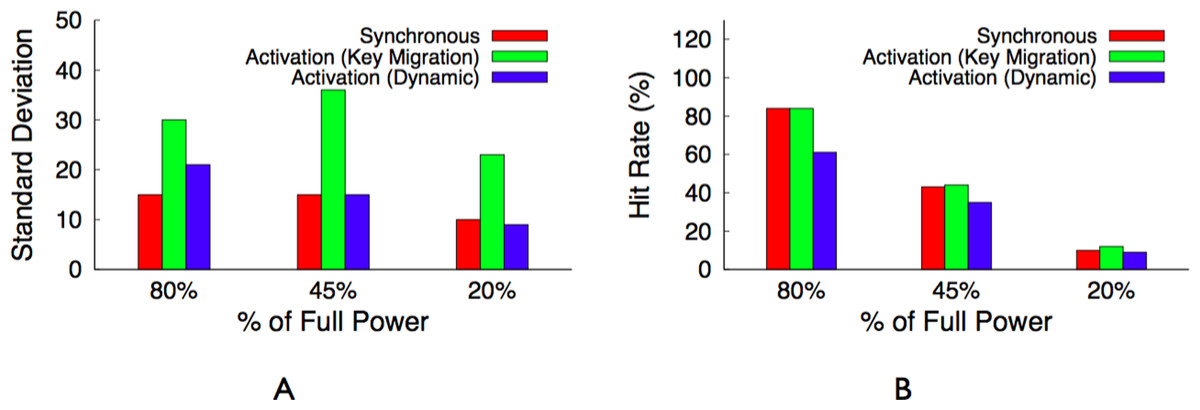
Figure 16: Comparison of fairness and hit rate with synchronous policy and activation policy for a uniform popularity distribution.
(A) Standard deviation with constant power. (B) Hit rate with constant power.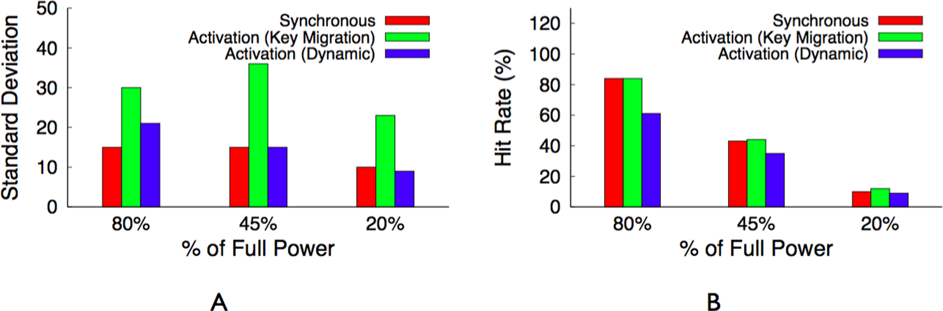
The synchronous policy is roughly 2X more fair than the activation policy with key migration at all power levels. While the dynamic hash-based mapping is nearly as fair as the synchronous policy, it has a worse hit rate, especially in high-power scenarios, as shown in Fig. 16B. Thus, the synchronous policy, which is more fair and provides lower average latency, is a better choice than any variant of the activation policy for uniform popularity distributions. Note that the key popularity distribution across servers in every memcached cluster that uses a hash-based mapping function is uniform, since keys map to servers randomly. Thus, the synchronous policy is the best choice for a heavily-loaded memcached cluster that cannot tolerate the throughput penalty of using proxies.
Balancing performance and fairness
Activation with key migration results in the maximum hit rate for skewed popularity distributions where some objects are significantly more popular than others, while the synchronous policy results in the best overall performance, in terms of both hit rate and fairness, for uniform popularity distributions. The proportional policy combines the advantages of both and works well for Zipf-like distributions with a few popular objects but a long tail of similarly (un)popular objects, since the long heavy tail in isolation is similar to the uniform distribution. Figure 17B shows the hit rate for the proportional policy, the activation policy with migration, and the synchronous policy for a Zipf popularity distribution with α = 0.6 at different power levels. The synchronous policy performs poorly, especially at low power levels, in this experiment, since it does not treat popular objects different than unpopular objects.
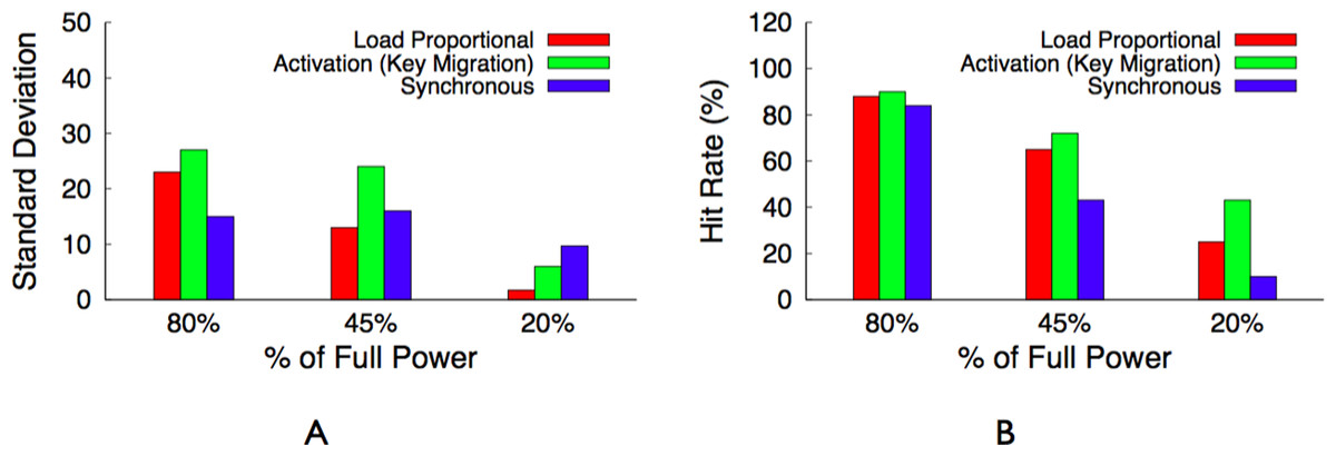
Figure 17: Comparison of fairness and hit rate with load proportional policy, synchronous policy and activation policy for a Zipf popularity distribution.
(A) Standard deviation with constant power. (B) Hit rate with constant power.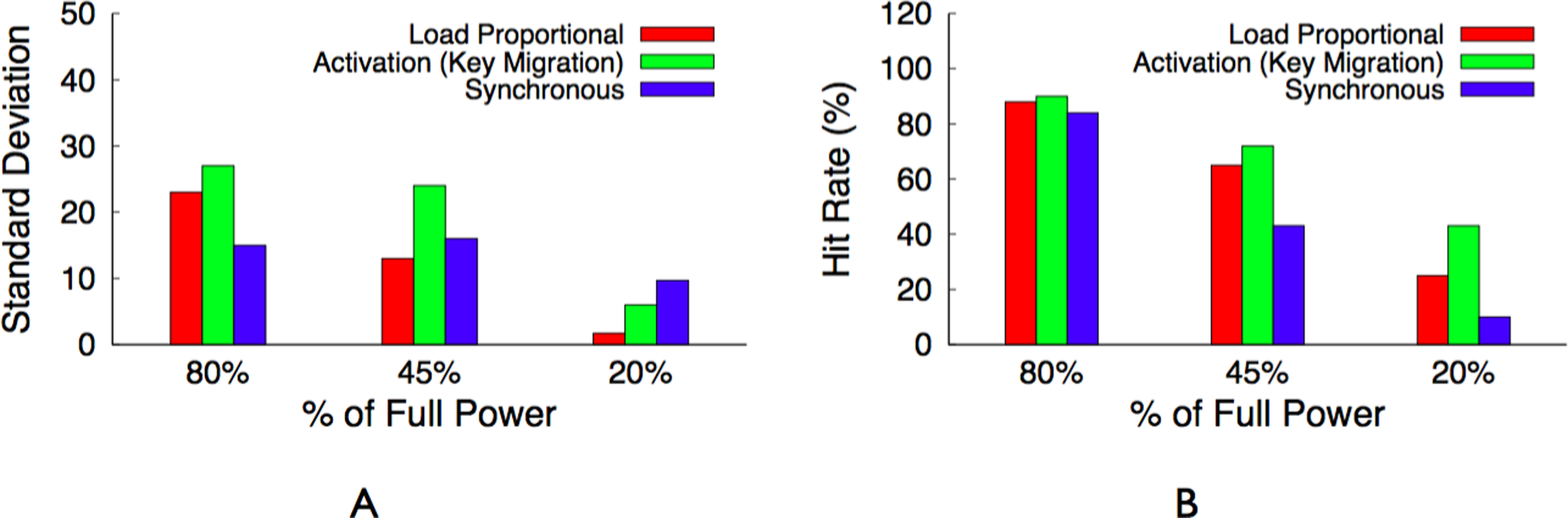
However, the proportional policy attains nearly the same hit rate as the activation policy at high power levels, since it also prioritizes popular objects over unpopular objects. Even at low power levels its hit rate is over 60% of the activation policy’s hit rate. Further, the proportional policy is significantly more fair to the many unpopular objects in the distribution. Figure 17A reports fairness, in terms of the standard deviation in per-object latency, at different power levels for the unpopular keys, i.e., keys ranked in the bottom 80th percentile of the distribution. The activation policy’s unfairness is nearly 4X worse at low power levels. Thus, the proportional policy strikes a balance between performance and fairness when compared against both the synchronous and activation policies.
Finally, Fig. 18 shows how the S3 transition overhead affects our results at a moderate power level. The figure shows that the overhead has only a modest effect on the load-proportional policy’s hit rate. The overhead does not affect the relative fairness of the policies. Note that all of our previous experiments use our prototype’s 2 s transition overhead. A shorter transition overhead would improve our results, and even a longer transition would show some, albeit lesser, benefits.
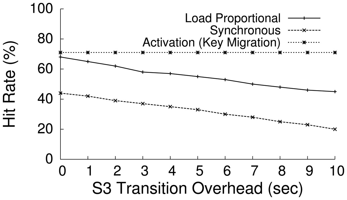
Figure 18: As S3 transition overhead increases, the hit rate from the load-proportional policy decreases relative to the activation policy with key migration for a Zipf distribution at a moderate power level.
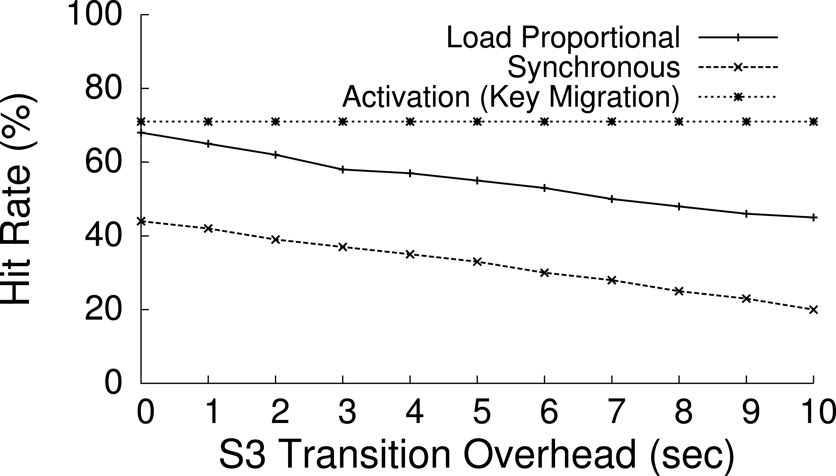
Case study: tag clouds in glassfish
While our prior experiments compare our blinking policies for different power and oscillation levels, we also conduct an application case study using traces from our energy harvesting deployment. The experiment provides a glimpse of the performance tradeoffs for realistic power signals. GlassFish is an open source Java application server from Sun, which includes a simple example application that reuses parts of the Java PetStore multi-tier web application, used in prior research, e.g., Cohen et al. (2004), to create tag clouds for pets. Tag clouds are a set of weighted tags that visually represent the most popular words on a web page. We modify the default web application to generate HTML for per-user tag cloud pages and cache them in memcached. The data to construct each HTML page comes from a series of 20 sequential requests to a MySQL database.
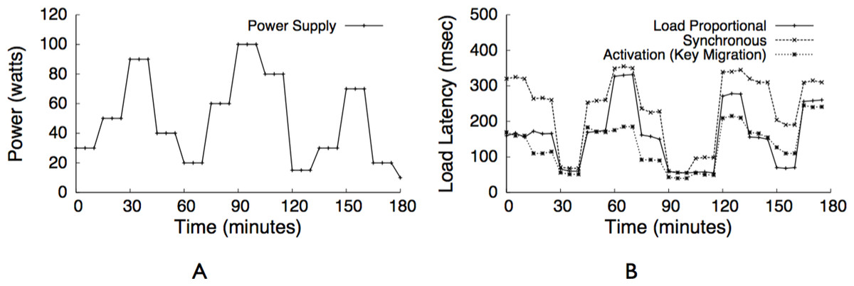
Figure 19: Power signal from a combined wind/solar deployment (A) and average page load latency for that power signal (B).
(A) Power. (B) Page Load Latency.
For these experiments, we measure the latency to load user tag cloud pages, which incorporates MySQL and HTML regeneration latencies whenever HTML pages are not resident in the cache. The MySQL latency for our simple table-based data is typically 30 ms per database query. While page load latency follows the same trend as hit rate, it provides a better application-level view of the impact of different policies. Figure 19B shows the average latency to load user web pages across 40,000 users for our three different policies—activation with key migration, proportional, and synchronous—for a combined solar and wind trace, assuming the popularity of each user’s tag cloud page follows a Zipf distribution with α = 0.6. We derive the power signal, shown in Fig. 19A, by compressing a 3-day energy harvesting trace to 3 h.
As expected, the activation policy with key migration and the load-proportional policy exhibit comparable page load latencies at most points in the trace. For this trace, the load-proportional policy is within 15% of the activation policy’s hit rate. The activation policy is slightly better at low energy levels, since it tends to strictly ensure that more popular content is always cached. Also as expected, the synchronous policy tends to perform poorly across all power levels. Also as expected, we measure the standard deviation of page load latencies for the load-proportional policy to be within 2% to the synchronous policy for the vast majority, i.e., bottom 80%, of the equally unpopular objects.
BlinkCache scalability
To see how our BlinkCache design performs for a large server cluster we use the Blink emulator from ‘Implementation’ to emulate a cluster of 1,000 nodes. We use the benchmark results from above to set the throughput, access latency, and power consumption of servers. As described above, each proxy can serve 10 memcached servers and give a maximum throughput of 1,000 requests/s. So, assuming the same throughput per proxy we select 100 proxies for our 1,000 node cluster which can give an aggregate maximum throughput of 100,000 requests/s. We use the same memcached client and request trace that we used for the evaluation of our real cluster.
As the number of proxies depend on the total number of active servers the activation policy activates/deactivates a number of proxies as it varies the number of active servers. To avoid migration of the key → server mappings from an inactive proxy to active ones we store all key → server mappings on each proxy. As each mapping requires only 20 bytes the overhead of storing all is minimal. A memcached client uses a simple mapping function—Hash(Key)%NumberProxies—to map a key to one of the proxies. If the number of active proxies changes a key previously mapped to a proxy might now map to a different proxy, which might not have the correct key → server mapping for that key. So, to reduce the overhead we sync the hash table (key → server mappings) of active proxies whenever their count changes.
First we evaluate the maximum throughput of the cluster at different power levels. As shown in Fig. 20 the maximum throughput increases linearly with the available power which dictates the maximum number of active nodes. Next, we evaluate the performance of aforementioned blinking policies—Activation with key migration, Synchronous, Load-proportional with key migration—at various steady and oscillating power levels. Comparing Fig. 21A with Fig. 17B it becomes clear that the performance (or relative performance) of different blinking policies does not vary much (within ±20%) with the cluster size. Further, the load-proportional policy performs better than the activation policy at high power for a large cluster, in construct to a small cluster of 10 nodes, as the key migration overhead dominates the performance gain due to keeping the popular keys on always-active servers for a large cluster at high power. But, like a small cluster, the performance gain dominates the migration overhead for the activation policy at low to medium power even for a large cluster. Figure 21B shows the hit rate for these three blinking policies for different oscillation levels from the 45% of full power. As expected, the hit rate for the activation policy drops down when the oscillation level increases because the migration overhead increases with the oscillation level. But, for the synchronous and load-proportional policies the hit rate remains the same at all oscillation levels because they don’t incur any migration overhead.
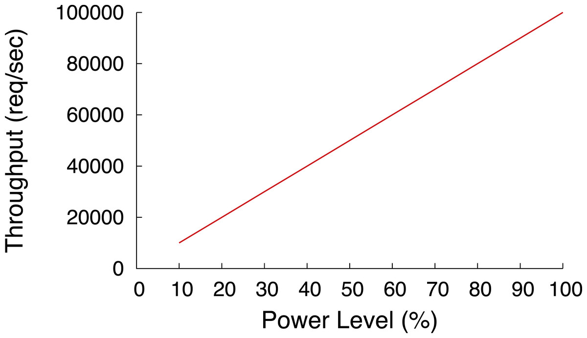
Figure 20: Throughput of a 1,000 node cluster with each node having the maximum throughput of 1,000 req/s.
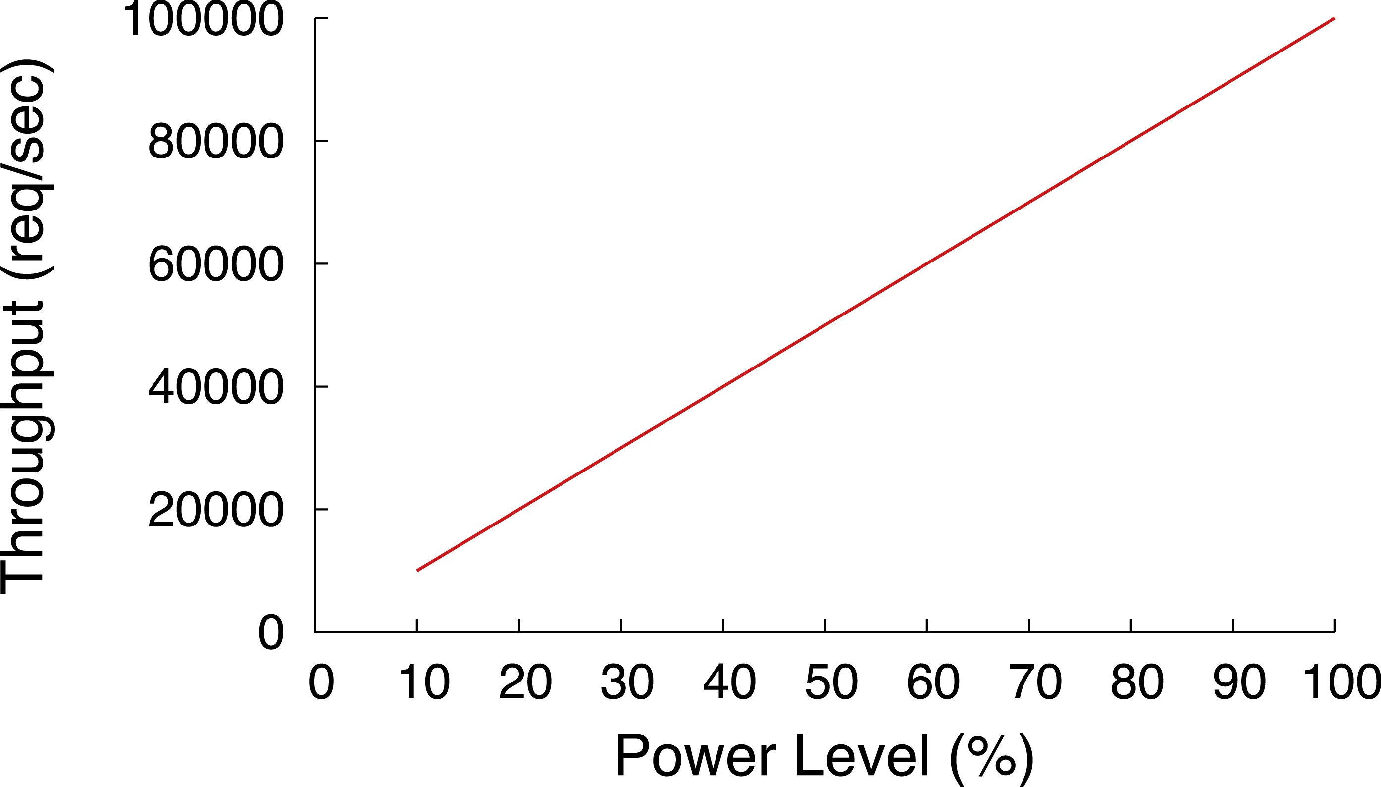
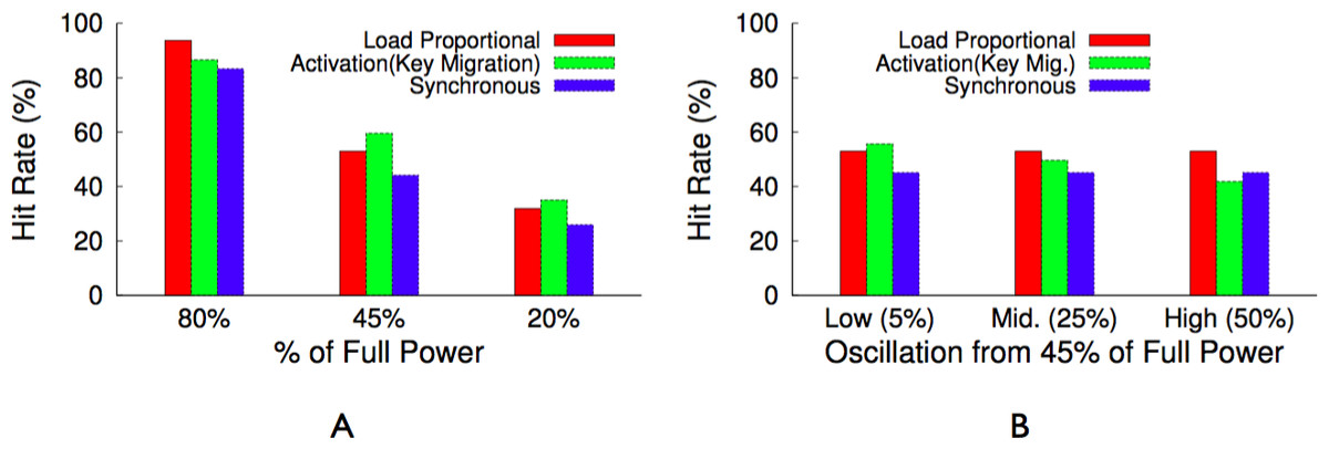
Figure 21: Comparison of hit rate with load-proportional policy, synchronous policy and activation policy for a Zipf popularity distribution.
(A) Steady power. (B) Oscillating power.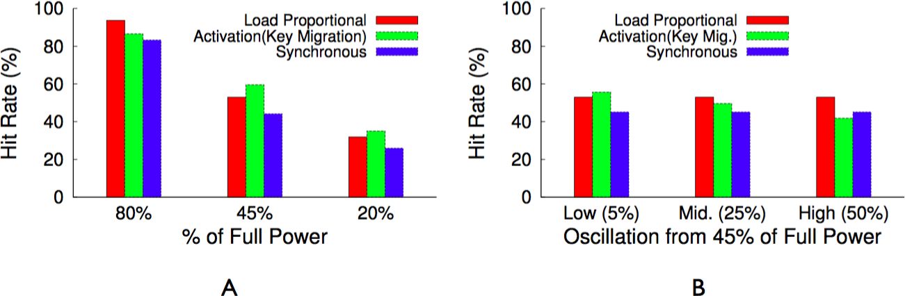
GreenCache evaluation
We first benchmark GreenCache’s proxy and chunking overhead for our prototype. We then evaluate GreenCache’s performance for real-world YouTube traces at multiple power levels with varying levels of oscillation. We then demonstrate the performance using realistic power traces from our energy harvesting deployment that have varying power and oscillation levels. We use two metrics to measure the performance: (1) bandwidth usage between the cache and YouTube servers and (2) average buffering or pause time at the clients. Bandwidth usage denotes the total data received from backend servers over a given time interval; it also represents bandwidth cost that mobile operators must pay to Internet service providers. One primary objective of GreenCache is to reduce this bandwidth usage. Another key objective of GreenCache is to improve user’s viewing experiences. Therefore, we consider average buffering time per video as our second metric to measure the performance. Note that our implementation tries to optimize both metrics independent of each other. However, optimizing for bandwidth usage does not depend on the power level, but on the total cache size, while optimizing for buffering time depends on both the cache size and the power level.
| Buffering time (s) | Power (%) | ||||
|---|---|---|---|---|---|
| ⇓ | 20 | 40 | 60 | 80 | 100 |
| Blink interval = 30 s | |||||
| Std Dev | 7.88 | 5.33 | 3 | 0.52 | 0.03 |
| 90th per | 21.25 | 15.25 | 9.25 | 2.25 | 0.23 |
| Avg. | 10.99 | 6.12 | 3.88 | 2.35 | 0.25 |
| Blink interval = 60 s | |||||
| Std Dev | 14.59 | 10.01 | 6.79 | 2.55 | 0.03 |
| 90th per | 41.25 | 28.25 | 19.25 | 7.45 | 0.23 |
| Avg. | 20.58 | 10.19 | 6.94 | 3.36 | 0.25 |
| Blink interval = 90 s | |||||
| Std Dev | 24.79 | 16.69 | 10.06 | 3.16 | 0.03 |
| 90th per | 66.25 | 43.25 | 25.65 | 4.25 | 0.23 |
| Avg. | 29.44 | 15.12 | 8.50 | 3.22 | 0.25 |
| Blink interval = 120 s | |||||
| Std Dev | 30.52 | 22.21 | 13.13 | 5.29 | 0.03 |
| 90th per | 78.25 | 59.45 | 31.45 | 14.45 | 0.23 |
| Avg. | 32.73 | 21.58 | 9.81 | 4.58 | 0.25 |
Benchmarks
To measure the proxy’s overhead, our client emulator creates a single thread and sends multiple video requests in succession. The breakdown of the latency overhead at each component for a sample 1 MB video chunk of 1 min play length, assuming a 135 Kbps bit rate, is 30 ms at the proxy, 20 ms at the cache server, 50 ms in the network between the proxy and cache server, and 100 ms in the network between the proxy and client. The result demonstrates that the proxy’s latency overhead is low. We also benchmark average buffering time for different blink intervals at various power levels. Table 5 shows the standard deviation, 90th percentile, and average buffering time for video requests, as the blink interval and power levels change. As expected, the buffering time increases with the blink interval at low to moderate power levels. We also benchmark the standard deviation, 90th percentile, and average buffering time for requests going to YouTube servers, which are as 150 ms, 570 ms, and 620 ms, respectively.
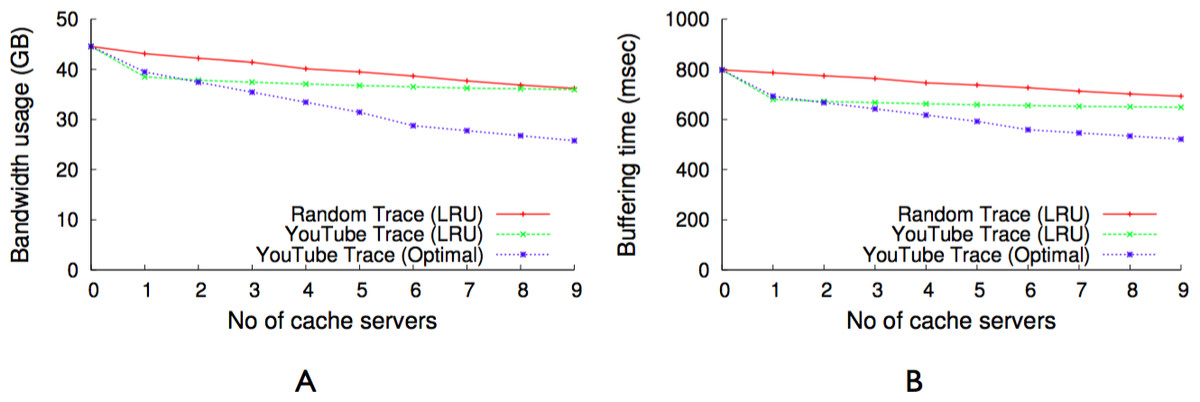
Figure 22: Both bandwidth usage and buffering time reduce with increasing cache size.
(A) Bandwidth usage. (B) Buffering time.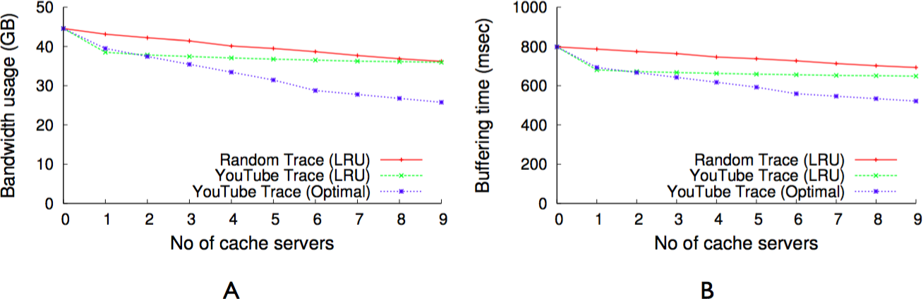
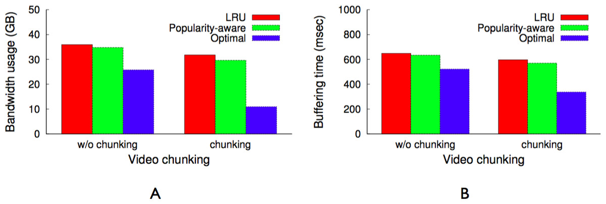
Figure 23: Video chunking reduces both bandwidth usage and buffering time.
(A) Bandwidth usage. (B) Buffering time.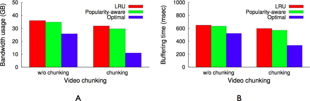
To study the performance of our prototype cache for different cache sizes and power levels we take a 3 h trace (from 7 PM to 10 PM on February 7th, 2012) from our 3 day YouTube trace. The trace contains a total of 8,815 requests, for 6,952 unique videos, over the 3 h interval. Our trace reports the URL, video ID, client IP address, and request time for each video. In addition, we pull the recommended list for each video in the trace from the YouTube servers. Based on the video ID, its recommended list, client IP address, and the next requested video ID, we calculate the viewing length for each video. We assume the average video length as 5 min and the streaming rate as 135 Kbps. Also, we fix the downlink bandwidth from backend YouTube servers to the WiMAX station to 1 Mbps, and the storage capacity of each cache server as 1 GB. Further, we fix the blink interval as 60 s. We use a weighing factor of 0.6 for the proposed popularity-aware eviction policy.
First, we study the performance—bandwidth usage and buffering or pause time for clients—for different number of cache servers at full power for the real world 3 h YouTube trace, as well as a synthetic trace of 8,815 requests where each request is for a randomly chosen video from the aforementioned 6,952 unique videos. In addition, we choose least-recently-used (LRU) cache eviction policy for this experiment; further, videos are not chunked. Figure 22 plots the total bandwidth usage and average buffering time for both random and real traces. We also plot the optimal performance for real traces assuming we know all requests in advance. The optimal policy always keeps most popular videos in the cache, and never evicts a popular video to store a less popular video (over a given interval). As expected, the total bandwidth usage and average buffering time over the 3 h interval decreases as the size or number of servers increases.
Next, to study the benefits of video chunking we measure the performance of three different cache eviction policies—LRU, popularity-aware, and optimal—for the 3 h real trace at full power and 9 cache servers. Figure 23 shows that the performance of GreenCache’s popularity-aware eviction policy is better (∼7%) than that of LRU. Further, video chunking improves (>15%) the performance of all policies as it avoids storing unpopular chunks of popular videos. In all cases, LRU performs worse than others, which motivates our use of a popularity-aware cache eviction policy and video chunking for all further experiments.
Staggered load-proportional blinking
As discussed earlier, the total bandwidth usage over a fixed interval, as long as a request does not go to backend servers for an already cached video, does not depend on the available power level or blinking and layout policies; it only depends on the cache size and eviction policies. However, buffering time and users’ experiences do depend on the available power, blinking and layout policies. In this section, we study the effects of the power level on the average buffering time, and various optimizations designed to reduce the buffering time. We use the same 3 h real YouTube trace, as discussed above, and 9 cache servers for all further experiments. Further, we use video chunking and the popularity-aware eviction policy for all experiments.
To compare the proposed staggered load-proportional policy with the activation and load-proportional policies, we also implement an activation policy and a load-proportional policy for GreenCache, and integrate them with GreenCache’s popularity-aware eviction policy, video chunking, and popularity-aware migration policy. The activation policy activates or deactivates servers as power varies, whereas the load-proportional policy distributes the power to servers in proportion to their popularity. Similar to the load-proportional policy, the activation policy also migrates popular chunks to active servers while deactivating servers due to the drop in the power level. Unlike the proposed staggered load-proportional policy, the load-proportional policy does not replicate video chunks because it does not benefit from replication as it activates all servers at the same time every blink interval.

Figure 24: Buffering time at various steady and oscillating power levels.
(A) Steady power. (B) Oscillating power.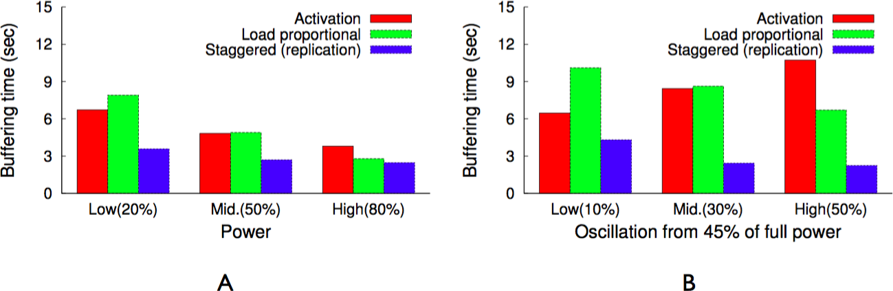
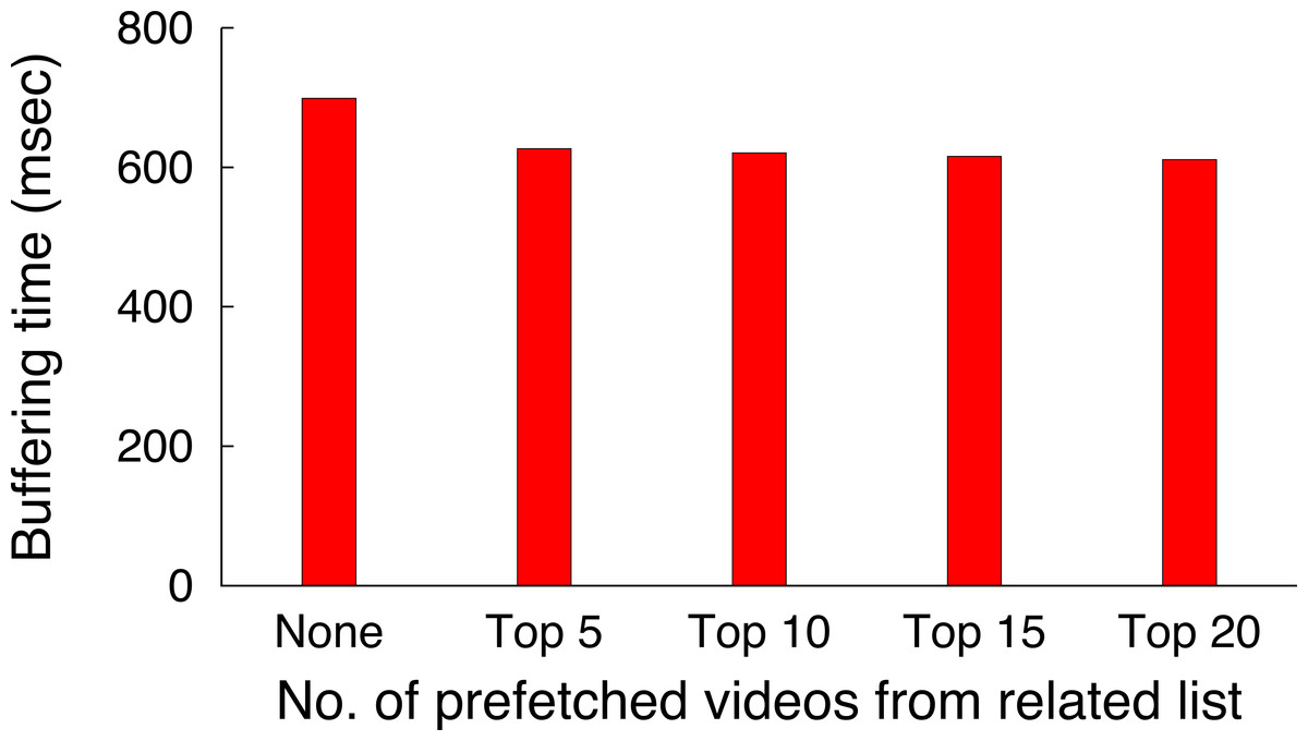
Figure 25: Buffering time decreases as the number of prefetched videos (first chunk only) from related lists increases.
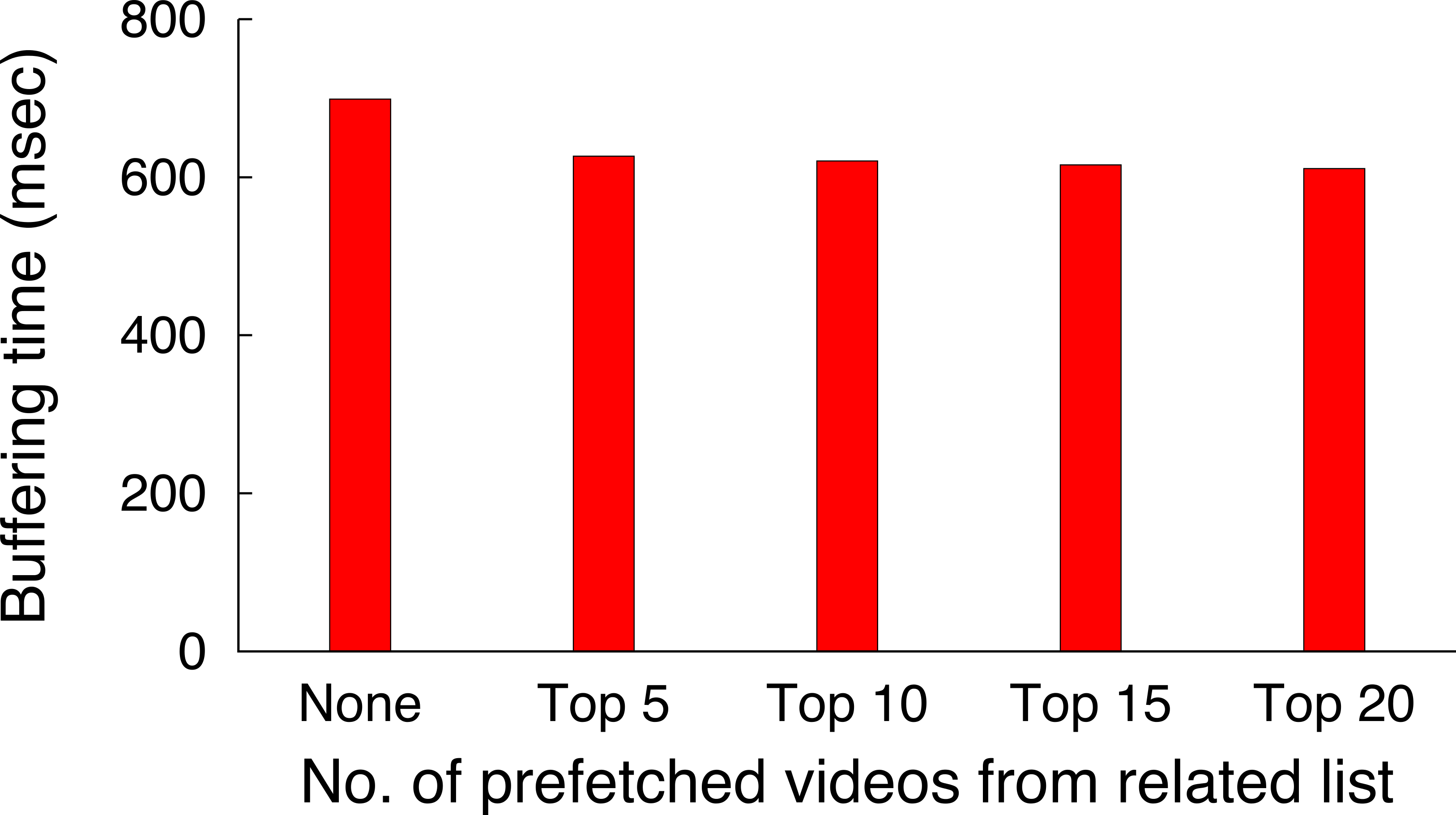
Figure 24A shows the average buffering time at different steady power levels. As expected, the activation policy performs better than the load-proportional policy at low power levels since, unlike the load-proportional policy, the activation policy does not incur the blinking overhead, which becomes significant in comparison to the active interval at low power levels. However, at moderate to high steady power levels, the benefit of a larger cache size, albeit blinking, dominates the blinking overhead for real-world traces. Furthermore, the buffering time decreases significantly if first chunks are replicated on all servers. Even at low power levels, replication of initial chunks significantly reduces the buffering time, while still leveraging the benefits of a larger cache size. Moreover, the performance of the staggered load-proportional policy remains almost the same at all power levels. As video popularity changes infrequently, migration overheads in our experiments are modest (∼2%).
Figure 24B compares the average buffering time for the above policies at different oscillating power levels. We oscillate available power every five minutes. Since migration overhead of the staggered proportional policy is independent of power level, its performance remains almost the same at all oscillation levels. However, the activation policy incurs migration overhead whenever the number of active servers decreases. Consequently, the activation policy performs poorly at high oscillation levels, as indicated in the figure. Though replication of initial chunks reduces the buffering time at all power levels, it is primarily required at low power levels.
Next, we evaluate the benefits of prefetching initial chunks of related videos. As Fig. 25 indicates, prefetching initial chunks of the top five videos reduces the buffering time by 10% as compared to no prefetching. Further, since prefetching more videos doesn’t improve the buffering time, we limit the cache to prefetching only first chunks of top few videos from the related list. We choose to prefetch top five videos only in order to strike a balance between the performance gain and prefetching overhead.
Case study
To experiment with our WiMAX base station using a real WiMAX client, we use a Linux Desktop with Intel Atom CPU N270 processor and 1 GB RAM connected to Teltonika USB WiMAX Modem. We disable all network interfaces except the WiMAX interface. The desktop connects to the WiMAX base station (NEC Rel.1 802.16eBS), which we configure to route all video requests from the desktop to the proxy. We replay the same 3 h YouTube trace on the WiMAX client, but we use real power traces from our solar/wind deployment, as described in the previous section, to power the GreenCache cluster.
Figure 26 plots average buffering time, calculated every five minutes, for three blinking policies: activation, load proportional, and staggered load proportional with first chunks replicated. As expected, the performance of all three policies goes down (buffering time goes up) when the available power drops down, and vice versa. However, the performance of activation degrades more than that of load-proportional when the available power drops down, since the activation policy incurs migration overhead when the number of active servers decreases. Further, replicating first chunks significantly reduces the buffering time for the staggered load-proportional policy at all power levels. Since the migration overhead of the staggered load-proportional policy is independent of power levels, its performance does not vary much, not even when the available power changes significantly, if first chunks are replicated.
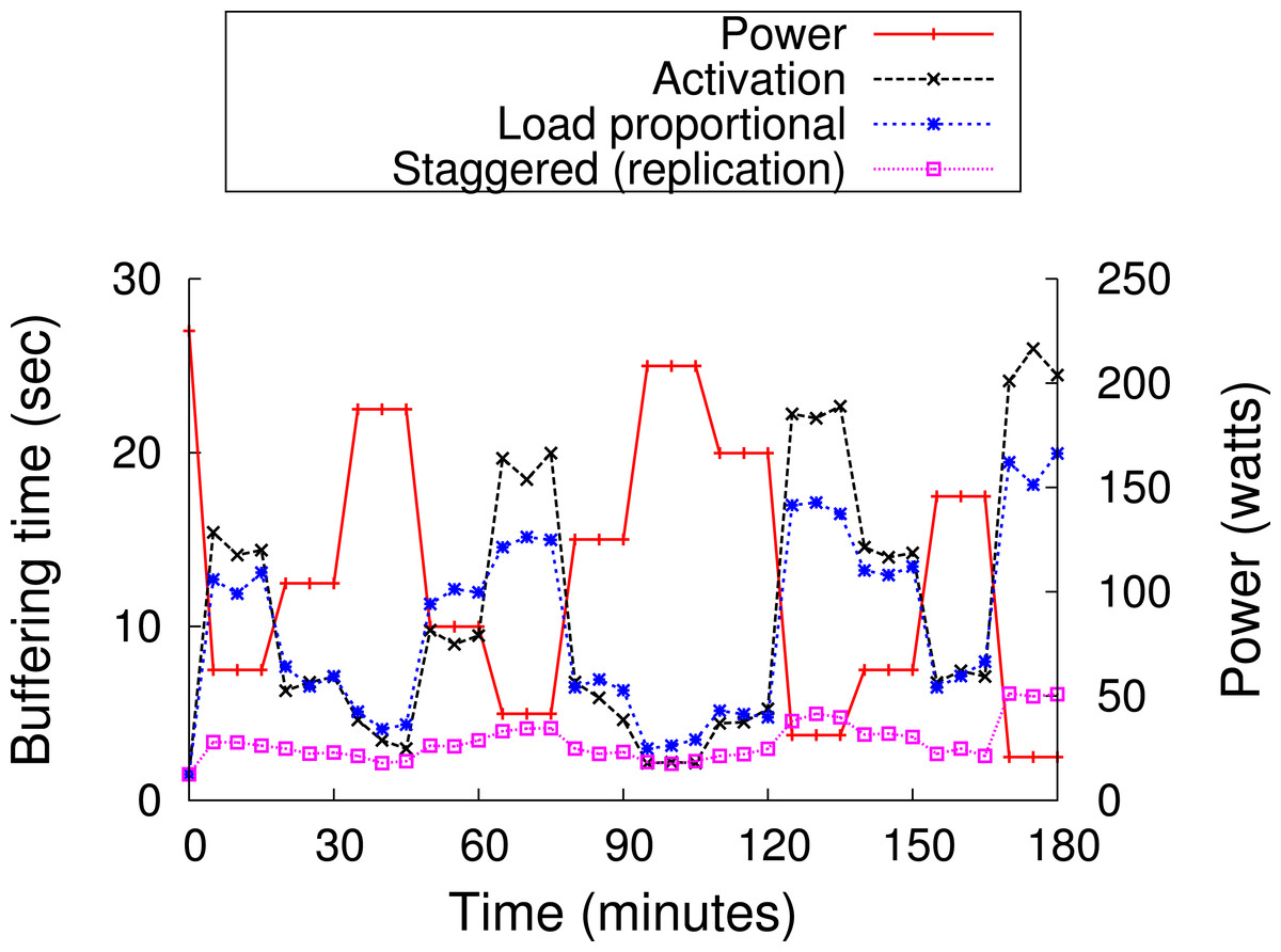
Figure 26: Buffering time at various power levels for our combined solar/wind power trace.
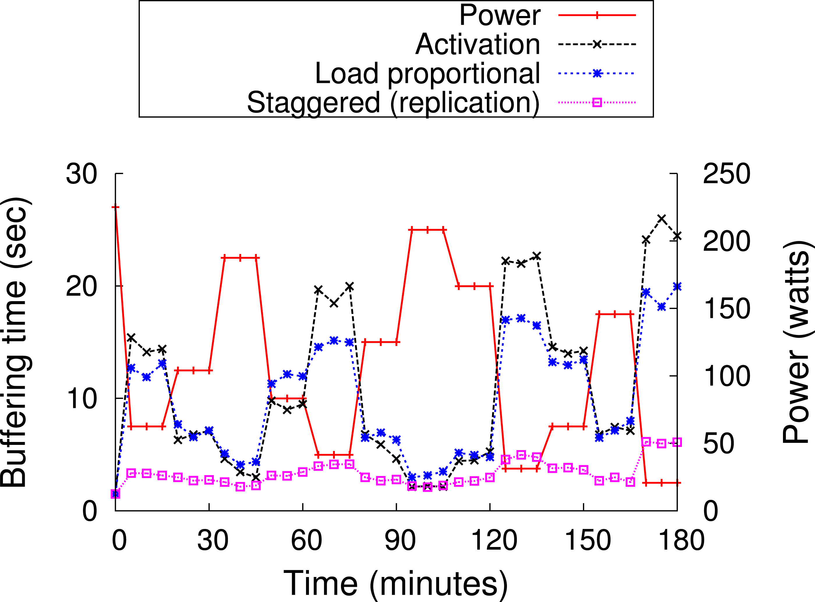
GreenCache scalability
Next, we use the Blink emulator to study how GreenCache performs on a cluster of 1,000 nodes for the YouTube dataset and user request trace described above. We run all Blink and GreenCache modules as described above, and use the benchmark results to set the throughput, access latency, and power consumption of servers. Figures 27A and 27B show the average latency and bandwidth, respectively, at various power levels. As expected, both the average latency and bandwidth cost reduce with increasing power levels as the number of active nodes or the total cache size increases with the power level.
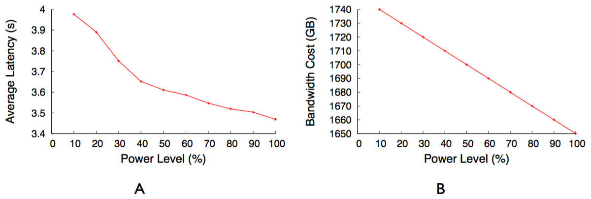
Figure 27: Latency and bandwidth cost on 1,000 node cluster for YouTube video requests with steady available power.
(A) Average latency in video requests. (B) Average bandwidth cost in video requests.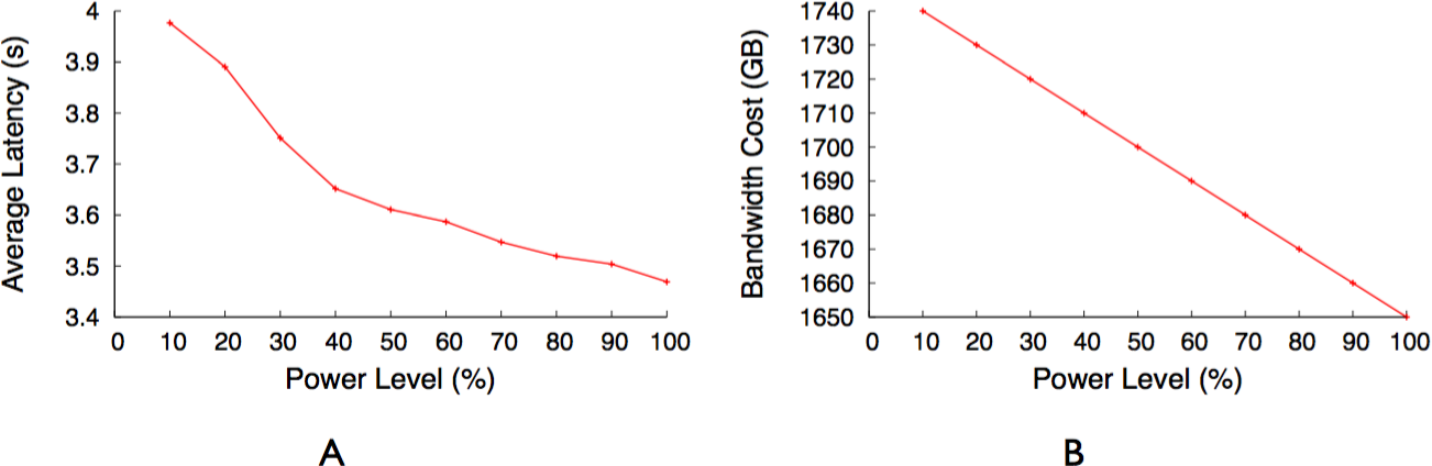
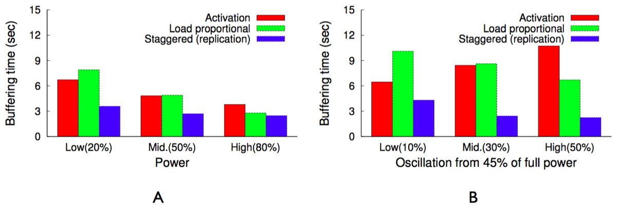
Figure 28: Buffering time with activation policy, load proportional policy, and staggered load proportional policy.
(A) Steady power. Oscillating power.
Figure 28A shows the buffering time for the aforementioned blinking policies at three different steady power levels. As expected, the staggered load-proportional policy performs best at all power levels due to the replication of first chunk of all videos. The load-proportional policy recalculates the popularity of chunks every 5,000 requests and migrates popular chunks to mostly active servers. Comparing Figs. 24A and 28A it is evident that the relative performance of different policies does not vary much with the cluster size. Similarly, Figs. 24B and 28B indicates that all three blinking policies give similar performance (or relative performance) for a small as well as a large cluster.
Related work
The sensor network community has studied strategies for dealing with variable sources of renewable power, since these systems often do not have access to the power grid. However, since sensor networks are geographically distributed, each node must harvest its own energy, resulting in network-wide energy imbalances (Fan, Zheng & Sinha, 2008), whereas data center nodes share a common power delivery infrastructure. Further, the primary performance metric for a sensor network is the amount of data the network collects. As a result, much of the energy harvesting work is not directly applicable to data centers. Similarly, mobile computing generally focuses on extending battery life by regulating power consumption (Zeng et al., 2002), rather than modulating performance to match energy production.
The increasing energy consumption of data centers (US Environmental Protection Agency, 2007) has led companies to invest heavily in renewable energy sources (Miller, 2008; Stone, 2007). For example, the goal of Google’s RE < C initiative is to make large-scale renewable power generation cheaper than coal-based production. As a result, researchers have started to study how to incorporate renewables into a data center’s power delivery infrastructure (Stewart & Shen, 2009). As one example, Lee et al. (2010) use request redirection to control the carbon footprint of data centers by redirecting load to servers powered by renewable energy sources. While not directly related to energy harvesting, Power Routing (Pelley et al., 2010) proposes shuffled power delivery topologies that allow data centers to control how much power each rack receives. While the topologies are well-suited for delivering variable amounts of power to racks based on aggregate demand, they are also useful for flexible routing of a variable power supply. Prior research on workload-driven approaches to improve data center energy efficiency is orthogonal to our work. Examples include designing platforms that balance CPU and I/O capacity (Anderson et al., 2009; Rivoire et al., 2008), routing requests to locations with the cheapest energy (Qureshi et al., 2009), and dynamically activating and deactivating nodes as demand rises and falls (Chase et al., 2001; Tolia et al., 2008; Krioukov et al., 2010). PowerNap’s node-level energy proportional technique has also been viewed as a workload-driven optimization (Meisner, Gold & Wenisch, 2009). We show that a similar technique is useful for controlling per-node power consumption in a power-driven system.
Power capping has also been studied previously in data centers to ensure collections of nodes do not exceed a worst-case power budget (Ranganathan et al., 2006; Fan, Weber & Barroso, 2007b). However, the work assumes exceeding the power budget is a rare transient event that does not warrant application-specific modifications, and that traditional power management techniques, e.g., DVFS, are capable of enforcing the budget. These assumptions may not hold in many scenarios with intermittent power constraints, as with our renewable energy power source. Gandhi et al. (2009) cap CPU power by forcing CPU idle periods. While similar, blinking focuses on capping per-node power where the CPU is only one component of the total power draw. Improving the energy-efficiency of storage is also a related research area. While Memcached does not offer persistent storage, our modifications for blinking adapt similar ideas from prior storage research, such as migrating popular objects to more active nodes (Pinheiro & Bianchini, 2004; Zhu et al., 2005a). Additionally, power-aware caching algorithms focus on maximizing the idle time between disk accesses to reduce disk power consumption, while our work focus on controlling the power consumption of the cache itself (Zhu et al., 2005b).
Blinking introduces regulated churn into data center applications as nodes switch from the active to inactive state. Churn has been well-studied in decentralized, self-organizing distributed hash tables (Stoica et al., 2001). However, the type of churn experienced by DHTs is different than the churn caused by blinking, which motivates our different approach to the problem. In the former case, nodes arrive and depart unexpectedly based on autonomous user behavior and network conditions, while in the latter case, nodes switch between the active and inactive states in a regular and controllable fashion. RAMCloud (Ousterhout et al., 2009) proposes using memory for low-latency persistent storage, and cites as motivation the increasingly large memcached clusters used in production data centers.
The use of caches to improve the performance of multimedia distribution systems has been studied extensively in the past two decades. Tang, Xu & Chanson (2005) gives a general overview on existing multimedia caching techniques. Due to the vast amount of exiting work in this area, we only focus on the work closely related to our approach, although, to the best of our knowledge, there is no existing work that directly addresses multimedia caches for intermittent power.
Wu, Yu & Wolf (2001) were among the first to propose the caching of chunks (segments) of a video. In contrast to our approach chunks are not equal in size and increase exponentially with the distance from the start of the video. The intention of this approach is to combine the number of consecutive chunks that are cached with the popularity of the video. E.g., for a very popular video all chunks would be stored on the cache while for less popular chunks only a certain number of the initial chunks of the video would be cached. Letting the chunk size grow exponentially has the advantage that the initial chunks of many videos can be stored without occupying too much of the caches storage space. Having only one or several initial chunks of a video stored on the cache bears the advantage that a requested video can be streamed to the client and played out without significant delay. Missing chunks can be streamed from the server immediately after the initial client request to allow for a smooth play out. In contrast to the approach presented by Wu et al., we decided for a scheme that splits all videos in equal sized chunks (except for the very last chunk) where the complete chunk can be transmitted to the client in a period that is equal or smaller than the blink interval, assuming a minimum transmission rate.
A more restrictive version of the caching of video chunks is the caching of the first chunk (prefix) only, which was introduced by Sen, Rexford & Towsley (1999). The sole goal of this approach is to reduce the buffer time at the client, since the first chunk can be streamed from the cache much faster than from a remote server. Our initial work on prefix prefetching of videos listed on YouTube’s related video list (Khemmarart et al., 2011) is based on this approach, but proactively prefetches prefixes instead of caching them. As we have shown in Khemmarart et al. (2011), prefix prefetching can significantly improve the viewer’s experience of watching videos and this motivated us to investigate how the prefetching approach performs on a multimedia cache for intermittent power. The results presented above show that prefix prefetching can improve the experience of a viewer also in the case of a blinking multimedia cache.
As in our current work, trace-based driven simulations are also used in Cha et al. (2007) and Zink et al. (2009) to investigate the effectiveness of caching for YouTube videos. Both investigations show that caching of YouTube video can both, on a global and regional level, reduce server and network load significantly. In contrast to the work presented in this paper, both studies do not consider scenarios in which power for the caches is intermittent.
Applicability of Blinking
While we apply blinking to two distributed applications in this paper, we believe blinking is applicable to other applications with intermittent power constraints. There are a range of scenarios beyond renewable energy where imposing intermittent constraints may be attractive. For example, data centers may wish to participate in automated demand-response programs with the electric grid. Automated demand-response, which is a cornerstone of a future smart electric grid, decreases power levels at participating consumers when the electric grid is under stress in exchange for lower power rates. Data centers are well-positioned to benefit from automated demand-response, since servers, as opposed to other types of electrical appliances, already include sophisticated power management mechanisms and are remotely programmable. Blink simply uses these pre-existing mechanisms to gracefully scale application performance as power varies. Additionally, data centers consume significant quantities of power, and demand-response programs typically target large power consumers first. Thus, addressing intermittent constraints in data centers may contribute to a more flexible and efficient electric grid.
In addition to automated demand-response programs, data center operators may wish to cap energy bills or power consumption at a fixed level for a variety of reasons, which also imposes intermittent power constraints. For instance, capping energy bills imposes variable power constraints when energy prices vary, as with wholesale energy prices which vary at intervals as low as every 5 min (Qureshi et al., 2009). Thus, as market prices vary, the amount of power a fixed budget purchases will also vary. Capping power is also necessary during “brownout” scenarios, more common in developing countries, where the electric grid is not always able to fully meet demand. Further, Ranganathan et al. (2006), as well as others (Fan, Weber & Barroso, 2007b), point out the benefits of oversubscribing a data center’s power delivery infrastructure, including the possibility of using dense clusters of lower-cost, but higher-power, components and then capping power to prevent damage.
Finally, we believe blinking is applicable to applications beyond memcached and multimedia cache. As with caches, applying blinking will likely require application-level modifications to handle regular and periodic disconnections. One particularly interesting case is leveraging blinking to run distributed storage systems under intermittent power constraints, such as in “brownout” scenarios. Persistent storage presents a different problem than caches, since there is not an alternative always-on option to fallback on to retrieve data. While we measure the performance of distributed caches primarily as a function of hit rate, a blinking storage system’s performance is primarily a measure of data availability, including both the latency and throughput to access data. As a result, a blinking storage system may need to judiciously replicate data to increase availability and ensure consistency across replicas, despite regular and frequent node transitions between the active and inactive states.
Conclusion
In this paper, we focus on managing server clusters running on intermittent power. We propose blinking as the primary abstraction for handling intermittent power constraints, and define multiple types of blinking policies. We then design an application-independent platform for developing and evaluating blinking applications, and use it to perform an in-depth study of the effects of blinking on two distributed applications—memcached and multimedia cache—for various power signals. We find that while an activation policy with key migration results in the best hit rates, it does not distribute the benefits of the cache equally among equally popular objects. As in-memory caches continue grow in size, they will store a greater fraction of equally popular objects for Zipf-like object popularity distributions. We propose and evaluate an asymmetric load-proportional policy to increase fairness without significantly sacrificing the cache’s hit rate. We then propose a staggered load-proportional policy that staggers the start time of servers to maximize the availability of at least one active server. Staggering the start time in conjunction with first chunk replication improves the performance of a multimedia cache, but it does not improve that of memcached because it is a key-value storage system and, unlike the multimedia cache, it does not stream data. We are currently studying how blinking applies to other types of data center applications, including distributed storage layers and data-intensive batch systems.