

Artificial neural network-based ground reaction force estimation and learning for dynamic-legged robot systems
- Published
- Accepted
- Received
- Academic Editor
- Bilal Alatas
- Subject Areas
- Artificial Intelligence, Autonomous Systems, Robotics, Neural Networks
- Keywords
- Legged robot, Ground reaction force, Estimation based on neural network, Supervised learning
- Copyright
- © 2023 An and Lee
- Licence
- This is an open access article distributed under the terms of the Creative Commons Attribution License, which permits using, remixing, and building upon the work non-commercially, as long as it is properly attributed. For attribution, the original author(s), title, publication source (PeerJ Computer Science) and either DOI or URL of the article must be cited.
- Cite this article
- 2023. Artificial neural network-based ground reaction force estimation and learning for dynamic-legged robot systems. PeerJ Computer Science 9:e1720 https://doi.org/10.7717/peerj-cs.1720
Abstract
Legged robots have become popular in recent years due to their ability to locomote on rough terrains; these robots are able to walk on narrow stepping-stones, go upstairs, and explore soft ground such as sand. Ground reaction force (GRF) is the force exerted on the body by the ground when they are in contact. This is a key element and is widely used for programming the locomotion of the legged robots. Being capable of estimating the GRF is advantageous over measuring it with the actual sensor system. Estimating allows one to simplify the system, and it is meant to be capable of prediction, and so on. In this article, we present a neural network approach for GRF estimation for the legged robot system. In order to fundamentally study the GRF estimation of the robot leg, we demonstrate our approach for a single-legged robot with a degree of freedom (DoF) of two with hip and knee joints on a flat-surface. The first joint is directly driven from the actuator, and another joint is belt-pulley driven from the second actuator to take advantage of the long range of motion. The neural network is designed to estimate GRF without attaching force sensors such as load cells, and the encoder is the only sensor used for the estimation. We propose a two-staged multi-layer perceptron (MLP) solution based on supervised learning to estimate GRF in the physical-world. The first stage of the MLP model is trained using datasets from the simulation, enabling it to estimate the simulation-staged GRF. The second stage of the MLP model is trained in the physical world using the simulation-staged GRF obtained from the first stage MLP as the input. This approach enables the second stage MLP to bridge the simulation to the physical world. The root mean squared error (RMSE) is 0.9949 N on the validation datasets in the best case. The performance of the trained network is evaluated when the robot follows trajectories that are not used in training the two-stage GRF estimation network.
Introduction
The ground reaction force (GRF) is one of the key elements used to control legged robots. GRF is used during robot locomotion for calculating control inputs in robot control systems. Cho et al. (2022) utilized GRF to estimate the ground contact state of the humanoid robot, LIGHT, in the control system. Other legged robots that utilize GRF for robot locomotion include GAZELLE (Jeong et al., 2020), Valkyrie (Radford et al., 2015), and Mini cheetah (Katz, Di Carlo & Kim, 2019). GRF needs to be measured or estimated to compensate for the external reaction forces by the control system. Azimi et al. (2018) described the disadvantages of implementing force sensors on a robot’s foot to measure GRF directly: (1) load cells are bulky and expensive; (2) load cells are difficult to mount on a robot because their dimensions; (3) load cells can fail due to overloading; (4) load cell measurements are often highly sensitive. There are some advantages to estimating GRF without force sensors: (1) no sensor issues like communication delay and calibration; (2) hardware design is no longer limited by the mounting position of sensors on foot; (3) model-based control systems (Miura & Shimoyama, 1984) are less affected by unmodeled sensor masses.
Some estimation methods were presented to estimate GRF in robots and humans. In Bobbert, Schamhardt & Nigg (1991), a computer vision-based method was presented to estimate the GRF of humans. Positions of human joints were captured with markers by cameras. The accelerations of each rigid body segment were calculated by video data to estimate GRF by Newton’s second law of motion. In Fakoorian et al. (2017), Kalman filter-based methods were presented to estimate the GRF of prosthetic legs. Two Kalman filter methods, which are continuous-time extended Kalman filter and unscented Kalman filter, were used. Both estimation methods are prone to diverge due to parametric uncertainties. In Azimi et al. (2018), a sliding mode observer (SMO) and an adaptive observer were presented to estimate the GRF of prosthetic legs. In order to ensure the effectiveness of the observer-based methods, it is essential to identify dynamic information about the system, such as mass matrix, Coriolis force, coulomb friction, and viscous friction.
A deep neural network is a good nonlinear regression models (Specht, 1991). Deep neural networks may be a good fit for nonlinear regression curves if data can be collected that contain the states of the robot and accurate GRF feedback. In Oh, Choi & Mun (2013), a neural network-based method was represented to estimate the GRF of humans. Kinematic states of humans were collected by a motion capture system, and preprocessed data was used in learning the GRF network. Neural network-based estimation methods have some advantages: (1) no need to know complex hardware parameters such as the tension of the belt, gear backlash, and static friction; (2) only simple matrix multiplication is executed so that the computational time is fast; and (3) the new training sets, which are not used in previous learning, can help the neural network to know the changed states in robots using online learning.
In this article, we propose a neural network-based fast GRF estimation method in a two-DoF (degree of freedom) point-foot robot. The entire end-to-end pipelines required to build a two-staged neural network for estimating GRF in a robot system are described. The first stage of the multi-layer perceptron (MLP) model estimates simulation-featured GRF, while the second phase of the model maps the featured GRF from the simulation environment to the physical world environment. The estimation performance of the learned GRF network (Fig. 1C) was compared with SMO (Azimi et al., 2018) (Fig. 1B). In addition, two different metrics were used to evaluate the regression performance of the proposed method. One is the root mean squared error (RMSE), which was used as a metric to show that the smaller the error, the smaller the residual between the estimate and the measured value. Another metric is R-squared, which shows better regression performance as the value approaches one and is more truthful and informative than other metrics used in regression methods (Chicco, Warrens & Jurman, 2021).

Figure 1: Our robot system for training the GRF estimation neural network.
(A) Our two-DoF point-foot robot with a linear guide and load cell (force sensor). (B) GRF estimation performance of SMO. (C) GRF estimation performance of the proposed method.
The contributions of this study are as follows:
1. A simulation to real (Sim2Real) approach is proposed to estimate the GRF that plays an important role in the locomotion of legged robots.
2. A two-staged MLP approach was proposed to bridge the domain gap between the simulation and the physical world and reduce overall training time.
3. The proposed method was implemented on a belt-pulley-driven legged robot, characterized by high model uncertainty caused by the variable tension of the belt. The proposed method demonstrated reliable estimation performance, even for non-trained motions.
The remainder of this article is organized as follows: “Related works” introduces related research about force estimation methods, MLP model, and Sim2Real methods; “System overview” describes the overall hardware system of the robot used in this paper. In “Training in the simulation”, we introduce how to collect training datasets and how to train the first stage MLP model in simulation; In “Transfer to the physical world”, training the second stage MLP is proposed to bridge the output of the first stage MLP to the physical world’s GRF. In “Whole process for GRF estimation”, we introduce the overall GRF estimation process in the physical world by using the proposed method and compare the proposed method with the observer-based method. “Conclusion and future work” summarizes the methods and proposes limitations and future works.
Related Works
Force estimation
Recent studies have investigated force estimation in various applications. In Azimi et al. (2018), researchers proposed two observer-based methods. Sliding mode observer and adaptive observer were proposed to estimate GRF in a powered three-DoF prosthetic leg. In Yigit et al. (2020), the authors used an observer-based method, an extended Kalman filter method, and an artificial neural network (ANN) trained with the physical-world datasets to estimate external force/torque in a variable stiffness actuator. Furthermore, a novel ANN-based method was proposed by Fallahinia & Mascaro (2022), which utilized a convolutional neural network to estimate the tactile grasp force of a human finger from image data. Other force estimation methods were proposed in Liu et al. (2018), Fakoorian et al. (2016), Sakamoto et al. (2023), Eguchi et al. (2019), and Xia & Kiguchi (2021).
MLP
In machine learning, MLP is a type of artificial neural network that consists of an input layer, one or more hidden layers, and an output layer. Each layer is made up of one or more nodes, also known as neurons, which perform a linear transformation of the input followed by a nonlinear activation function. MLP is a versatile tool and can be utilized for many tasks, such as classification, regression, and feature extraction. With the increasing depth of neural networks in deep learning, MLPs are also widely used due to their flexibility and effectiveness.
In addition, MLP is an artificial neural network that can be used for capturing complex and nonlinear relationships between input and output variables (Specht, 1991; Hornik, Stinchcombe & White, 1989). With sufficient training data and computational resources, MLPs can approximate the highly nonlinear function with high precision. MLPs are made up of interconnected layers of nodes, where each node applies a nonlinear activation function to the weighted sum of its inputs. These functions allow the MLP to learn complex and nonlinear transformations of the input data. While training an MLP model, the MLP adjusts the weights and biases of its nodes to minimize a loss function that measures the difference between the model’s estimations and the ground-truth values of the output variable.
In regards to robot control, the appropriate selection of activation function, number of layers, and number of nodes are essential for fast and accurate estimation with MLP. The activation function plays a significant role in determining how the neurons in each layer transform the input data. The nonlinearity and smoothness of various activation functions can impact the accuracy and speed of MLP’s output estimation. While a highly nonlinear activation function can effectively capture complex patterns in the data, it increases the computation burden. Besides, the number of layers and nodes in the MLP architecture are essential factors that influence estimation speed and performance. A deeper network with more layers can potentially capture more complex relationships in the data, but this may come at the expense of increased computation time. Similarly, increasing the number of nodes in each layer may enhance the model’s nonlinearity, but it may also raise the risk of overfitting and slow down the estimation speed.
Overall, MLPs are a versatile and potent tool for nonlinear regression, capable of capturing complex relations in the given data and providing reliable estimations when their parameters are tuned to ensure optimal performance for a specific task.
Sim2Real
Sim2Real is an approach that involves training an artificial neural network in a simulated environment and transferring it to a physical world environment. This method aims to reduce the time and cost associated with training neural networks while maintaining optimal performance in the real world. However, one of the main challenges of Sim2Real is the domain gap between the simulation and the physical world environments (Höfer et al., 2021), which can result in decreased performance when the trained network is used in the physical world. To address this challenge, domain randomization and domain adaptation are two main approaches used to overcome the issue of domain gap.
Domain randomization is a technique that involves randomizing parameters such as textures, masses, and dynamics during the simulation. This approach exposes the model to various conditions it might encounter in the physical world, making it more robust and better equipped to handle unexpected situations and variations. The ultimate goal is to enhance the model’s credibility in the physical world by allowing it to learn to adapt to different environments through domain randomization. In Peng et al. (2018), dynamics randomization is applied to develop reinforcement learning policies that adapt to highly different dynamics to overcome modeling errors in the physical world.
Domain adaptation is used to bridge the gap between the simulation and the physical world environments by adapting the knowledge learned from the simulation to the physical world. Domain adaptation involves re-training the trained network with datasets collected in the physical world to learn the discrepancies between the two environments. In domain adaptation, feature-based methods, instance-based methods, and adversarial methods are included. In feature-based domain adaptation, the aim is to learn features that are invariant to both domains. Instance-based domain adaptation uses a few labeled examples from the target domain to modify the model to the target domain. Adversarial domain adaptation focuses on training a model to make the two domains indistinguishable, thereby enabling the model to generalize well to the physical world. In Ganin et al. (2016), the adversarial domain adaptation method was applied to train an artificial neural network to not classify the domain while maintaining high performance in both domains.
System overview
In this section, we present the overall hardware configuration, including a point-foot robot and sensors, for GRF estimation. Figure 1A shows our point-foot robot, which has two-DoF with hip/knee joints connected to a linear guide for motion stability, and the parameters and coordinate definition of the robot are respectively shown in Table 1 and Fig. 2B. In order to reduce the mass of the links, we used stiff, lightweight aluminum as the material for the thigh/calf links. Two planetary reduction geared motors were used as actuators for the two joints, and the motor specifications are shown in Table 2. The actuator for the hip joint was directly connected to the output side of the motor. In contrast, the actuator for the knee joint was connected to the motor with a timing belt, which was aligned with the hip motor to reduce inertia. Figure 2A shows the structure of the timing belt system in the robot. We set up the radius and number of teeth to be equal for the input and output pulleys so that the speed ratio was 1:1. Figure 3 shows the overall communication system in our robot for training a GRF estimation network. CAN communication was used to connect the motor driver to the control PC at a frequency of 1 kHz and a bitrate of 1 Mbps. The load cell was used to measure the physical world’s GRF. Serial communication was used to obtain measured GRF at a frequency of 1 kHz.
| Parameters | Value | Unit |
|---|---|---|
| mbase | 2.948 | kg |
| mthigh | 0.349 | kg |
| mcalf | 0.303 | kg |
| l1 | 0.23 | m |
| l2 | 0.23 | m |
| q1 | −180∼180 | degree |
| q2 | −160∼160 | degree |
| Pulley radius | 0.039 | m |
| Belt length | 0.705 | m |
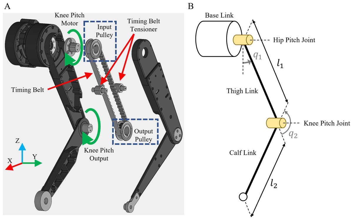
Figure 2: Configuration of the robot.
(A) Structure of the belt-pulley driven part of the robot. (B) Coordinate definition of the robot.
| Parameters | Value | Unit |
|---|---|---|
| Gear ratio | 1:9 | – |
| Mass | 0.710 | kg |
| Rotor inertia | 0.00034 | kgm2 |
| Nominal speed | 122 | rpm |
| Max speed | 160 | rpm |
| Nominal torque | 13 | Nm |
| Max torque | 45 | Nm |

Figure 3: Overall communication system for the control and measure the GRF of the robot.
The timing belt and pulley mechanism reduced the inertia while locating the actuator position far from the joint position. In this regard, sufficient belt tension was required to transmit the rotational force generated by the motor using the belt. The tension works to distribute the rotational force, so it can be regarded as the static friction between the two different pulleys. Therefore, the timing belt and pulley mechanism affected the actuating model by friction and tension of the belt and is not affected by the backless of the planetary gear in the motor. This effect resulted in the difference between the simulation model and the real hardware model. This difference was regarded as the difference as a domain gap for the Sim2Real problem.
Including the specific reason mentioned above, various and un-modeled cause GRF differences between the ground truth and the estimated value obtained from the equation of the motion. Figure 1B shows data collected in real experiments which highlight these differences. It is important to focus on this phenomenon and to resolve it in the simple dynamic model for the legged system.
The GRF estimation proposed in this article was based on the neural network trained with the data collected in a simulation environment and the real world. As opposed to the ideal data collecting condition in a simulation environment in terms of high sampling frequency and none of noise, data collected in real experiments are limited by the following conditions: The maximum bandwidth of the data is limited by the specification of the sensor system collecting GRFs, including the load cell, the processor of the analog to digital converter (ADC), etc. Also, the data contains sensor noise. For these reasons, the sensors used to measure the robot’s motion and the ground contact forces may not provide enough information to accurately estimate the GRFs.
Training in the simulation
In this section, we described how we collected data from the robotics simulation (Hwangbo, Lee & Hutter, 2018) and trained the GRF estimator using the collected datasets with PyTorch C++ API (Paszke et al., 2019). We selected the MLP model as the estimation model and chose the appropriate training parameters. We also evaluated the performance of the trained GRF estimator in the simulation.
Collecting datasets
In collecting the training datasets in the simulation, it was assumed that the joint positions, velocities, and torques could be measured. The desired height of the robot from the ground () is set as sinusoidal functions as described in Eq. (1). Inspired by the Fourier series, which can express all conceivable motions as a combination of sinusoidal functions, the amplitude (hA), frequency (f), and offset (h0) were varied to produce a diverse range of robot motions while collecting datasets. The constraints on each parameter in the sinusoidal function are set as Eq. (2). (1) (2)
In Eq. (3), the analytic inverse kinematics method was used to derive the desired states of each joint () based on the generated desired height of the robot () while adhering to kinematic constraints.
(3)
We used a joint PD controller (Eq. (4)) as a motion controller to track the desired joint states of the robot. (4)
During the simulation, the robot’s states (Eq. (5)) and measured GRF (Eq. (6)) were collected for supervised learning with a sampling frequency of 1 kHz. A total of 1,303,309 datasets were collected. Of the collected datasets, 90% were used for training the model and the remaining 10% for the validation of the trained model. The overall framework for collecting datasets is shown in Fig. 4. (5) (6)
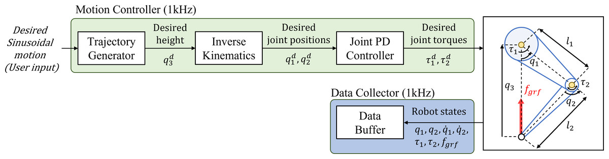
Figure 4: Framework for collecting datasets in the simulation.
Training MLP model
The MLP network model was chosen for the GRF network due to its lower computational burden compared to other models, such as the convolutional neural network (CNN). The overall hierarchy of the MLP network model for GRF estimation is illustrated in Fig. 5.

Figure 5: Hierarchy of the MLP network model for GRF estimation.
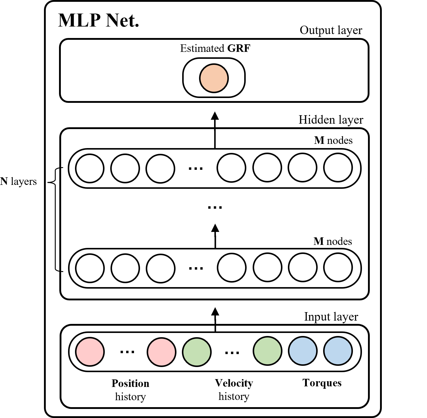
The input layer of the network was comprised of histories of joint positions and velocities, as well as current joint positions, velocities, and torques. According to Hwangbo et al. (2019) in ‘Modeling the actuation’, two histories with a time interval of 20 ms were selected to learn the network’s dynamics.
The hidden layer of the MLP network consisted of three major components: (1) the number of hidden layers (represented as N in Fig. 5); (2) the number of nodes (represented as M in each layer); and (3) the type of activation function in each layer. These components had a crucial role in the estimation time and performance of the trained network. If MLP networks are trained with large values of M and N, they can easily overfit and require significant time for estimation. Additionally, the type of activation function also affects the calculation time and performance of the trained networks. Hence, the careful selection of these three components is crucial to ensure that the trained network fit our system.
The training of the MLP network followed Algorithm 1 in Table 3. To achieve higher performance, we used the adaptive batch size algorithm based on ADABATCH (Devarakonda, Naumov & Garland, 2017), which gave a higher performance associated with large batches, maintaining the better test accuracy of small batches. For faster convergence, we chose the Adam optimizer (Kingma & Ba, 2014). The batch size was updated twice and the checkpoint was lowered when the model’s loss fell below the checkpoint. The training process stopped when the current number of epochs reached 300.
| Algorithm1: Adaptive Batch Size Learning Algorithm | |
|---|---|
| In | Datasetstraining |
| Out | Model |
| 1 | BatchSize = 16 |
| 2 | Epochmax = 300 |
| 3 | Checkpoint = 0.1 |
| 4 | repeat |
| 5 | executeSupervisedLearning withOptimizerAdam, Datasetstraining |
| 6 | ifModelLoss < Checkpoint then |
| 7 | Checkpoint←0.75∗Checkpoint |
| 8 | BatchSize←2∗BatchSize |
| 9 | Epoch←Epoch + 1 |
| 10 | untilEpoch < Epochmax |
To discover an appropriate MLP model for GRF estimation, we employed supervised learning using different types of activation functions and varying numbers of hidden layers and nodes. The experiments were conducted on 18 different models, and the results are presented in Table 4. RMSE on validation datasets and single estimation time were measured for performance evaluation.
| MLP Model | Activation function | Num. of layers | Num. of nodes | RMSE | Estimation time |
|---|---|---|---|---|---|
| 1 | softsign | 3 | 8 | 0.0024 N | 455 µsec |
| 2 | softsign | 3 | 16 | 0.0008 N | 462 µsec |
| 3 | softsign | 3 | 32 | 0.0004 N | 468 µsec |
| 4 | softsign | 9 | 8 | 0.0009 N | 560 µsec |
| 5 | softsign | 9 | 16 | 0.0005 N | 566 µsec |
| 6 | softsign | 9 | 32 | 0.0003 N | 599 µsec |
| 7 | softsign | 27 | 8 | 0.0016 N | 878 µsec |
| 8 | softsign | 27 | 16 | 7.5123 N (failed) | − |
| 9 | softsign | 27 | 32 | 7.5385 N (failed) | − |
| 10 | swish | 3 | 8 | 0.0005 N | 472 µsec |
| 11 | swish | 3 | 16 | 0.0002 N | 494 µsec |
| 12 | swish | 3 | 32 | 0.00006 N | 503 µsec |
| 13 | swish | 9 | 8 | 0.0003 N | 617 µsec |
| 14 | swish | 9 | 16 | 0.00008 N | 627 µsec |
| 15 | swish | 9 | 32 | 0.00004 N | 661 µsec |
| 16 | swish | 27 | 8 | 0.0002 N | 818 µsec |
| 17 | swish | 27 | 16 | 0.00009 N | 915 µsec |
| 18 | swish | 27 | 32 | 0.00009 N | 995 µsec |
In the MLP models tested, those utilizing the swish activation function displayed lower RMSE values compared to those utilizing the softsign activation function. The estimation time for the swish activation function models was slightly longer. However, the difference in estimation time between models with the same number of layers and nodes but different activation functions ranged from only 17 to 61 µsec, which does not significantly affect the control system. Additionally, results from model 8 and model 9 indicated that utilizing the softsign activation function with a relatively large number of layers and nodes failed to produce successful learning. Thus, utilizing swish as the activation function in the hidden layer is recommended.
In order to determine the optimal number of layers for the GRF estimation network, we compared the results of model 10 to model 18. From our analysis, we discovered that the RMSE decreased as the number of layers increased up to nine, but increased when it exceeded that number. Additionally, we observed that the estimation time increased proportionally to the number of layers. Based on these findings, we selected nine layers as the optimal number for the network’s performance.
After determining the number of layers, we proceeded to select the optimal number of nodes by comparing model 13, 14, and 15. There was a trade-off between the error and estimation time as the number of nodes increased. However, even in model 15, which used 32 nodes, the estimation time was only 661 µsec, indicating that about 1,500 estimates can be conducted in a second. This was sufficient for our control system, which had a control frequency of 1 kHz.
As a result, we chose model 15 as our GRF estimation MLP network, as it utilized the swish activation function, had nine layers, and 32 nodes in each layer. This model was determined to provide the optimal balance between estimation accuracy and computational efficiency for our specific control system. (The performance of the selected model is shown in bold in Table 4).
GRF estimation in the simulation
In order to evaluate the performance of the trained GRF estimator, we conducted experiments to estimate GRF using the trained MLP network in the simulation for various robot motions. The overall process to estimate GRF in the simulation is shown in Fig. 6A. During the estimation of GRF in the simulation, the robot’s states were sampled at a rate of 1 kHz and stored in the state buffer. From the state buffer, the time-series states of the robot were fed into the input of the trained network. The trained model outputs the estimated GRF at each time period.
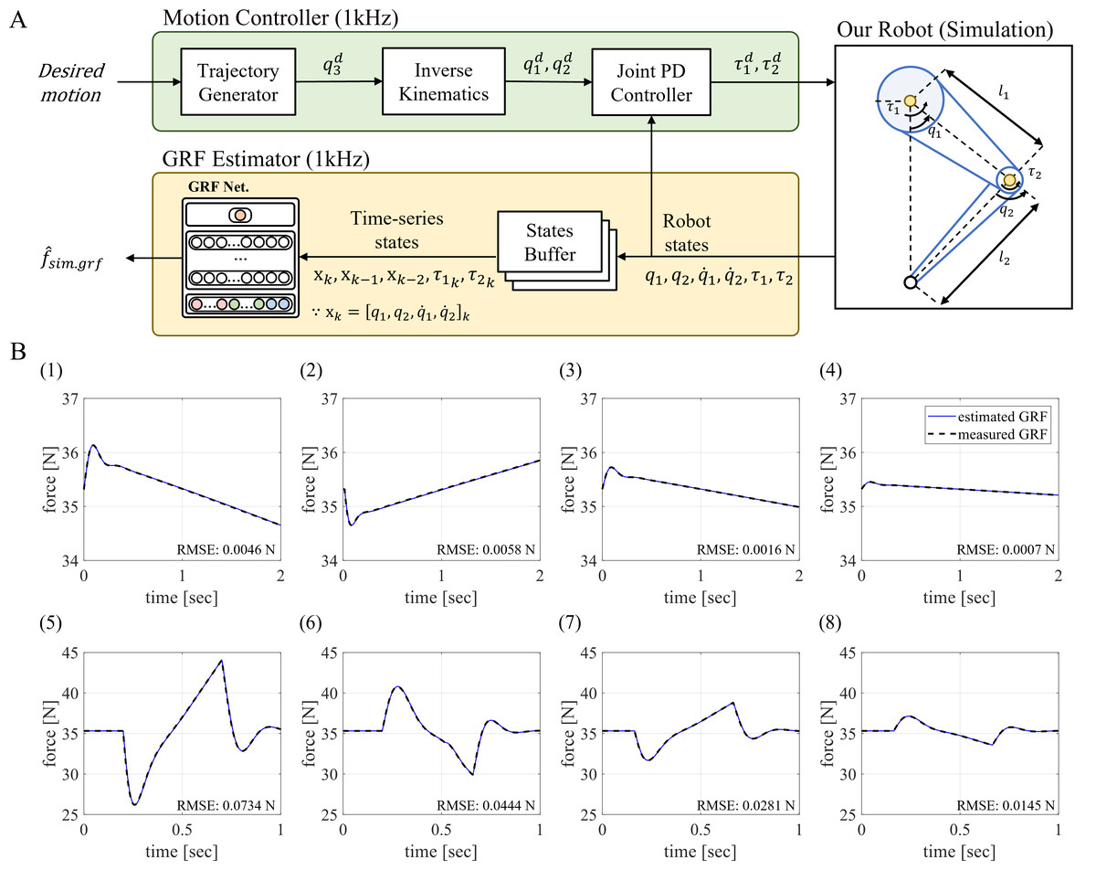
Figure 6: Estimation of the GRF in the simulation.
(A) Overall GRF estimation process in the simulation. (B) GRF estimation performance of the trained MLP network in the simulation with different cubic motions.
The trained GRF estimator was evaluated in different cubic motions that were not used in training. The results of the experiments are shown in Fig. 6B. In Fig. 6B, cases (1) to (4) are the results of GRF estimation when the robot followed the cubic polynomial trajectories to the target position in 2 s. Cases (5) to(8) are GRF estimation results when the robot moves in a relatively short time of 0.5 s. From the results, the RMSEs are less than 0.1 N in all cases, indicating that the estimation performance of the trained network was satisfactory.
The results of the experiments demonstrated that the proposed GRF estimator performed sufficiently for the different cubic motions, implying its ability to estimate GRF for non-trained motions. In addition, the trained MLP network, which was trained on motions generated using the Fourier Series-inspired strategy, has the ability to estimate GRF for a wide range of motions.
Transfer to the physical world
In this section, we present the strategy used to employ the GRF estimation network, which was trained with the simulation in the physical world scenarios. We evaluated the performance of the network when directly applied to the physical world, and we introduced a Sim2Real approach that aims to bridge the gap between the simulation and the physical world.
Naive Sim2Real transfer
We attempted to naively estimate the GRF in the physical world by employing the GRF estimator trained with the simulation datasets. The procedure to estimate GRF in the physical world has the same process as the estimation of GRF in the simulation and is depicted in Fig. 7A. The point-foot robot was controlled in a 1 kHz closed-loop, and the robot’s states were sampled at the same frequency. These sampled states were saved in the states buffer; the time-series states were fed into the trained network as input, and the output of the network is estimated GRF. The results of the naive estimation method are shown in Fig. 7B.
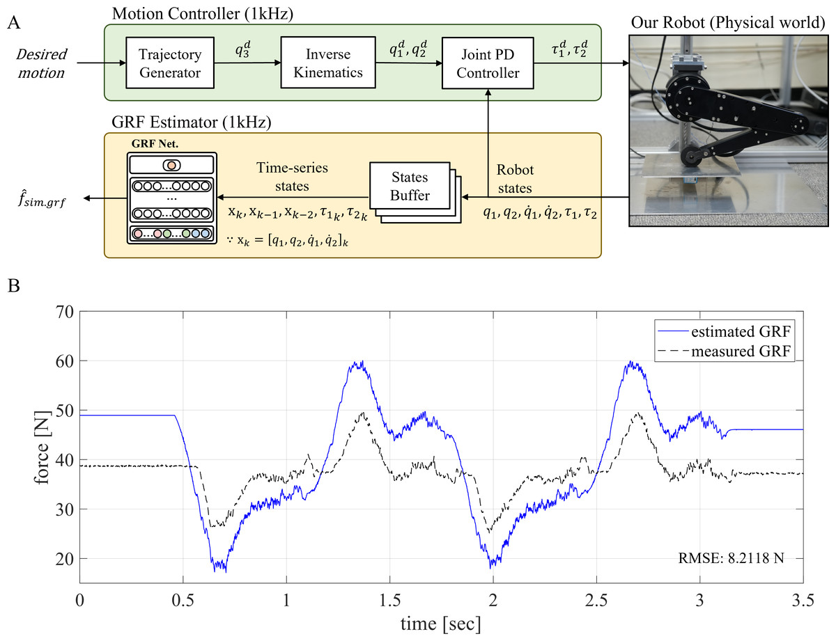
Figure 7: Naive estimation of the GRF in the physical world.
(A) Overall GRF estimation process of the naive Sim2Real approach. (B) GRF estimation performance of the naive Sim2Real approach.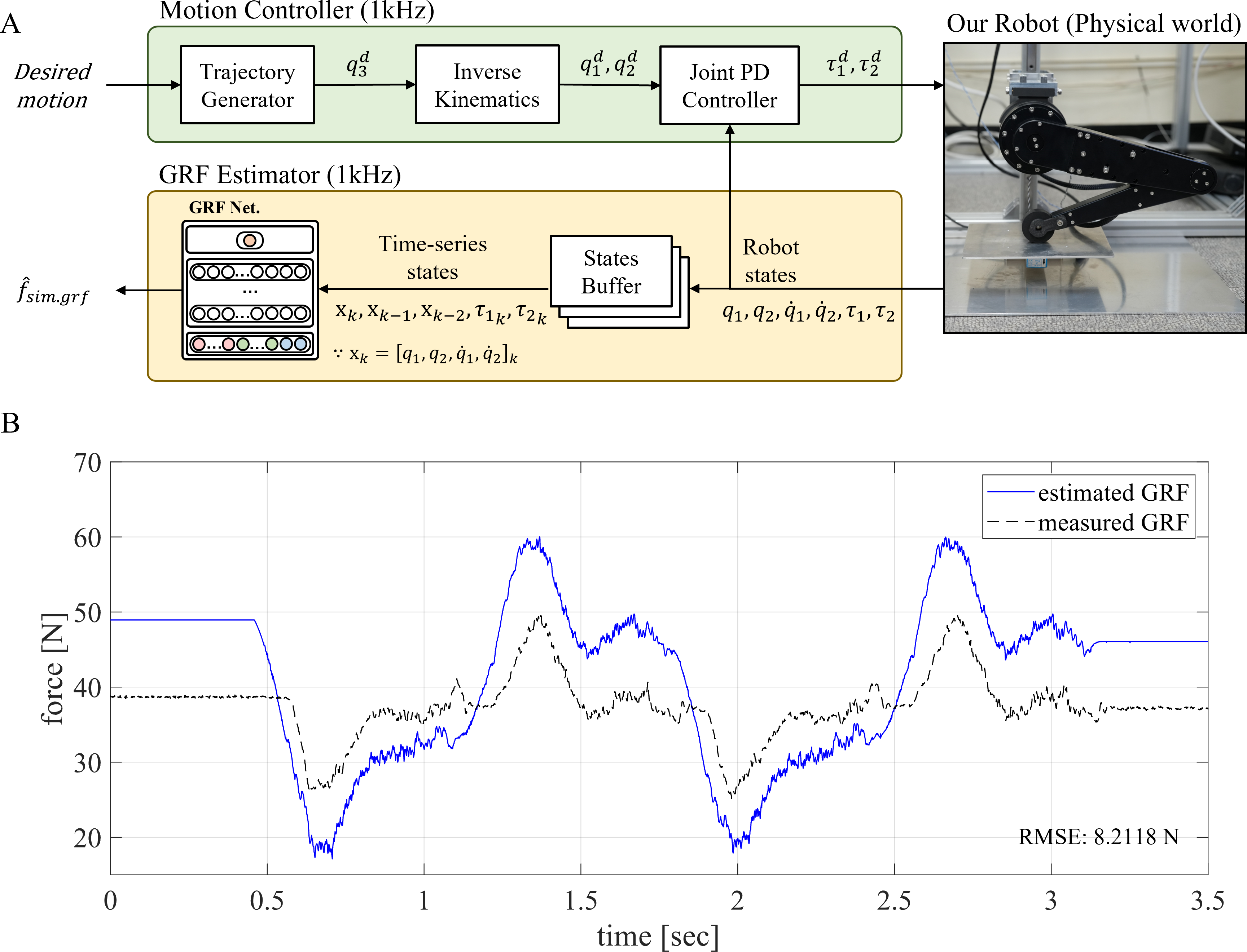
In the naive Sim2Real approach, the RMSE was 8.2118 N on the given robot motion. This performance was attributed to the domain gap, which included mechanical features such as gear backlash, static friction, torsional stress, and unmodeled wires for communication and power distribution. Despite the GRF estimator’s unsatisfactory performance, the estimated GRF still followed the overall profile of the measured GRF, which indicated that the peak values occur simultaneously. In other words, the trained network learned the relationships between the time-series robot states and GRF but had nonlinear offsets.
We propose using an additional neural network directly after the GRF estimation network to bridge the domain gap in order to overcome the domain gap between the simulation and the physical world.
Sim2Real bridge network
To train an additional network to bridge the estimated GRF to the physical world, we first measured the GRF from the physical world using a load cell.
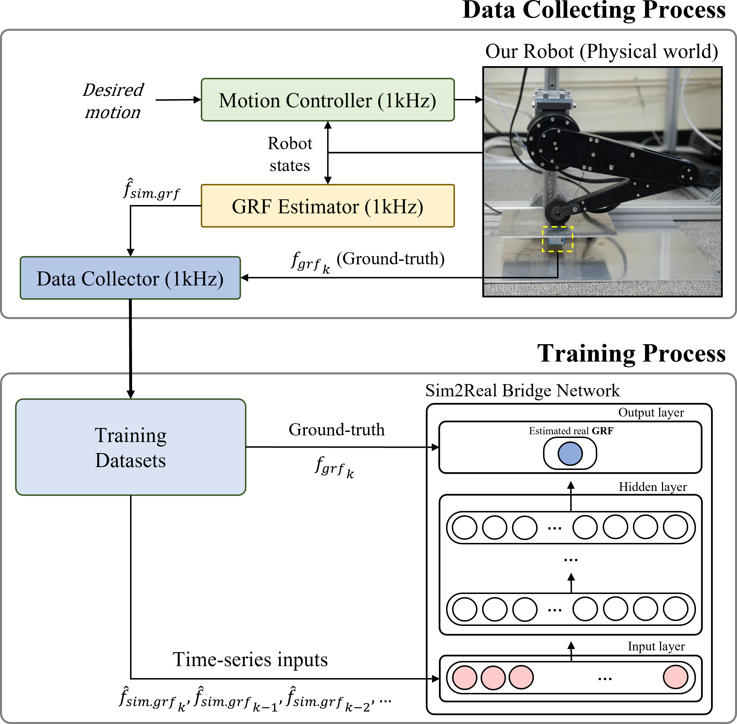
Figure 8 shows the overall framework from the data collection process to the training process of the Sim2Real bridge network. Estimated GRFs were collected as the inputs of the Sim2Real bridge network from the GRF estimation network. The measured forces were collected to use as ground-truth for the output of the Sim2Real bridge network. A total 131,968 datasets were collected in nine different sinusoidal motions. The entire process of collecting real-world datasets was completed in three minutes.
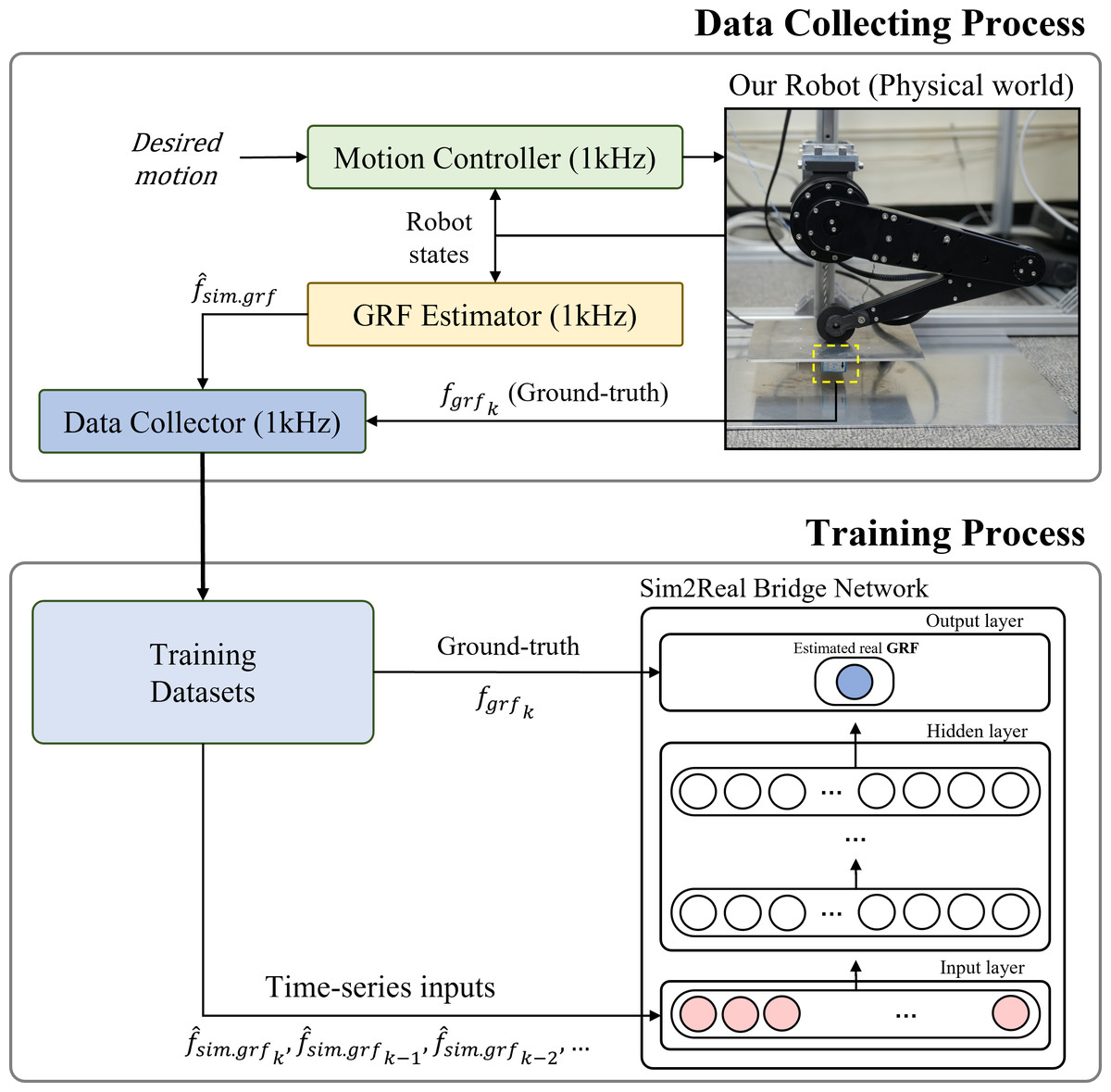
Figure 8: Overall framework for training Sim2Real bridge network.
The physical robot’s state contained noise components caused by sensors such as encoders, which were for measuring joint positions and velocities. In addition, delays exist in the physical world, which are caused by communication between PC and motor drivers, while the simulation has no delay induced by communication. Because of the noise and delay in the inputs of the GRF estimation network, the estimated GRF also contains noise components.
To address these hindrances in the training process of the bridge network, we decided to use time-series estimated GRF as input to teach system characteristics to the bridge model. In addition, we determined the amount of time-series data that was needed to teach the model the system characteristics. For training the Sim2Real bridge network, the hierarchy of the MLP model was fixed with six hidden layers and eight nodes, utilizing the swish activation function. The Adam optimizer was employed to update the weights of the MLP model. To determine the appropriate time-series input, we conducted experiments with the different combinations of interval time and the number of time-series.
A total of 20 combinations of time-series inputs were tested, and the training results are shown in Table 5. In the models that used five time-series inputs with different interval times, MSE decreased when the interval time increased. However, in the models that used 20 time-series inputs, the best case was when the interval time was 20 msec. Likewise, in the cases with the same interval time but different numbers of time-series inputs, the tendency of MSE as similar to the previous case. The best-case occurred when the number of time-series inputs was 50 and the time interval was 10 msec. In order to lower the number of the inputs for the fast estimation of the model, a model that uses 20 number of time-series and 20 msec time interval was selected for the Sim2Real bridge network. (The performance of the selected model is shown in bold in Table 5).
| Number of time-series | ||||
|---|---|---|---|---|
| Interval time | 5 | 10 | 20 | 50 |
| 1 msec | 2.1057 | 2.1293 | 2.0285 | 1.8863 |
| 5 msec | 1.8093 | 1.5758 | 1.8392 | 1.1082 |
| 10 msec | 1.6429 | 1.2863 | 1.2527 | 0.9923 |
| 20 msec | 1.4347 | 1.2853 | 0.9949 | 1.1016 |
| 50 msec | 1.1464 | 1.1332 | 1.0569 | 1.1284 |

Figure 9: Estimation of the GRF in the physical world.
(A) Whole framework to estimate GRF using the two-staged MLP network in the physical world. (B) Estimation performance of the two-staged MLP network and SMO in different four motions.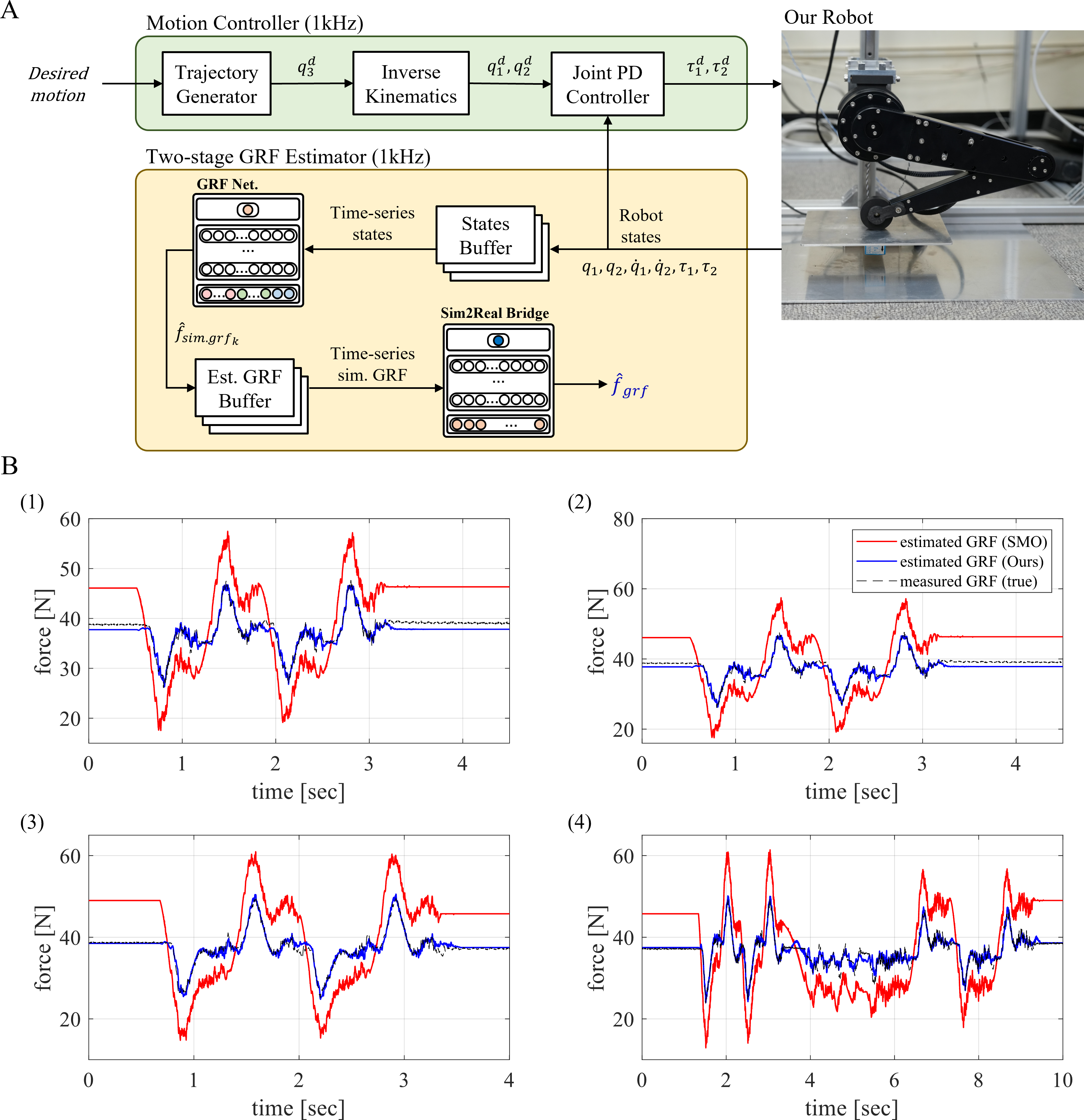
Process for GRF estimation
This section presents the process for estimating GRF in a point-foot robot in the physical world. The overall block diagram for GRF estimation is shown in Fig. 9A. The motion controller generates control inputs in a 1 kHz feedback loop for the given motion, and the robot’s states were saved to the states buffer for generating time-series states for the GRF estimation network in the two-staged GRF estimator. The output of the GRF estimation network was also saved to the buffer and used as the time-series inputs of the Sim2Real bridge network. Finally, the Sim2Real bridge network estimated the physical world’s GRF of the robot. The proposed two-stage neural network’s GRF estimation performance in the physical world is shown in Fig. 9B and was compared with the observer-based method. Table 6 provides a comparison and evaluation of the GRF estimation performance using the proposed method with the observer-based method. The evaluation includes two metrics, RMSE and R-squared. RMSE resulted in a lower value at 1.2094, and R-squared had a value closer to 1 at 0.8791, indicating that the proposed method had a better estimation performance than the observer-based method.
| Estimator | RMSE | R-squared |
|---|---|---|
| Proposed method | 1.2094 | 0.8791 |
| SMO | 8.6625 | −5.2004 |
Conclusion and Future Work
In this article, we proposed a GRF estimation method based on supervised learning using a two-staged MLP network in the belt-pulley-driven legged robot, which has high model uncertainty. Compared with the observer-based GRF estimation method, the proposed GRF estimation network showed better estimation performance. Instructions were provided for collecting datasets to train the MLP network used to estimate GRF in various motions in the robot. In order to collect datasets covering the various bandwidth of motion, we generated motion inspired by the Fourier series. The datasets were suitable to estimate GRF for various leg motions and were verified. In addition, pipelines for the estimation of GRF using a two-staged MLP network were proposed. The first stage of MLP estimated simulation level GRF and the second stage of MLP was trained for transferring the simulation level GRF to the physical world. This approach is a cost-effective method as it requires less data collection time and places lower strain on the robot hardware compared to existing methods that solely rely on actual data for learning contact force. Limitations of the proposed method arise when applied to flat-foot robots due to the significance of the contact configuration of the foot. In flat-foot robots, the center of pressure on the foot changes during contact with the ground. The performance of the proposed method in flat-foot robots cannot be assured without information about the center of pressure. In the future, we will improve the performance of the Sim2Real bridge model to lower the loss for the robustness of the estimation. Using our approach on a higher dimensional system with multiple legs and a floating-based body may show the feasibility of our approach in support of the improved performance of the learning model. On the other hand, we will apply the trained GRF network in dynamic planning for acrobatic motions and develop a force control system based on the GRF estimator in the legged robot systems so that our approach works well for the dynamic planning problem.