
Effective attributed network embedding with information behavior extraction
- Published
- Accepted
- Received
- Academic Editor
- Yilun Shang
- Subject Areas
- Artificial Intelligence, Data Mining and Machine Learning, Data Science, Network Science and Online Social Networks, Social Computing
- Keywords
- Attributed networks, Network embedding, Information behavior features, Topic-based community features
- Copyright
- © 2022 Hu et al.
- Licence
- This is an open access article distributed under the terms of the Creative Commons Attribution License, which permits unrestricted use, distribution, reproduction and adaptation in any medium and for any purpose provided that it is properly attributed. For attribution, the original author(s), title, publication source (PeerJ Computer Science) and either DOI or URL of the article must be cited.
- Cite this article
- 2022. Effective attributed network embedding with information behavior extraction. PeerJ Computer Science 8:e1030 https://doi.org/10.7717/peerj-cs.1030
Abstract
Network embedding has shown its effectiveness in many tasks, such as link prediction, node classification, and community detection. Most attributed network embedding methods consider topological features and attribute features to obtain a node embedding but ignore its implicit information behavior features, including information inquiry, interaction, and sharing. These can potentially lead to ineffective performance for downstream applications. In this article, we propose a novel network embedding framework, named information behavior extraction (IBE), that incorporates nodes’ topological features, attribute features, and information behavior features within a joint embedding framework. To design IBE, we use an existing embedding method (e.g., SDNE, CANE, or CENE) to extract a node’s topological features and attribute features into a basic vector. Then, we propose a topic-sensitive network embedding (TNE) model to extract a node’s information behavior features and eventually generate information behavior feature vectors. In our TNE model, we design an importance score rating algorithm (ISR), which considers both effects of the topic-based community of a node and its interaction with adjacent nodes to capture the node’s information behavior features. Eventually, we concatenate a node’s information behavior feature vector with its basic vector to get its ultimate joint embedding vector. Extensive experiments demonstrate that our method achieves significant and consistent improvements compared to several state-of-the-art embedding methods on link prediction.
Introduction
Network embedding (NE) aiming to map nodes of networks into a low-dimensional vector space, has been proved extremely useful in many applications, such as node classification (Perozzi, Al-Rfou & Skiena, 2014; Tang et al., 2015), node clustering (Cao, Lu & Xu, 2015), link prediction (Grover & Leskovec, 2016). A number of network embedding models have been proposed to learn low-dimensional vectors for nodes via leveraging their structure and attribute information in the network. For example, spectral clustering is an early method for learning node embedding, including models such as DGE (Perrault-Joncas & Meila, 2011), LE (Wang, 2012) and LLE (Roweis & Saul, 2000). Matrix decomposition is another important method for learning node embedding, for example, GraRep (Cao, Lu & Xu, 2015) and TADW (Yang et al., 2015). Spectral clustering and matrix decomposition embedding methods usually have high computational complexity with the increasing network size. In recent years, various network embedding methods have been proposed using random walk-based methods, which are faster and more effective, including DeepWalk (Perozzi, Al-Rfou & Skiena, 2014), Node2Vec (Grover & Leskovec, 2016), LINE (Tang et al., 2015), and SDNE (Wang, Cui & Zhu, 2016). More recently, deep learning and attention mechanisms are used to generate network embeddings, including GCN (Kipf & Welling, 2016), GAT (Veličković et al., 2018) and CANE (Tu et al., 2017), which extract structure, text, topic, and other heterogeneous feature information more effectively. In addition to the above methods, a few role-based approaches of network embedding (Jiao et al., 2021) have been proposed recently, where a role-based network embedding (Zhang et al., 2021) captures the structural similarity and the role information. Nevertheless, these methods are all limited with focusing on the network topological structure and attributed information while ignoring the implicit relationship between information. In reality, information has interactive behavior in some real-world networks such as social networks and citation networks, where the nodes have information behavior (Pettigrew, Fidel & Bruce, 2001), including information inquiry, information access, and information sharing. Therefore, we introduce the concept of informational behavior to deal with the information interaction. In real-world social networks and citation networks, it is intuitive that all of the nodes naturally prefer to interact with similar nodes. In this way, the exchange and sharing of information between nodes are more efficient, which is also the reason for the formation of various topic networks communities. For example, due to different majors, three topic-based communities, C0, C1, and C2, have been formed (as illustrated in Fig. 1). In these communities, nodes interact within both intra-community (such as nodes v0 and v3) and inter-community (such as nodes v0 and v1, v1 and v2, v2 and v3). This means that one node may communicate and share information in various topics when interacting with neighboring nodes of different communities and build bridges among nodes that are not directly connected, such as nodes v1 and v3 may have a link because nodes v0 or v2 acts as a bridge, but this link is not observed. It can be seen that these information behaviors are very important features, and the representation vectors for nodes without information behavior features are incomplete. However, these existing embedding methods are not able to cope with the information behavior of nodes.
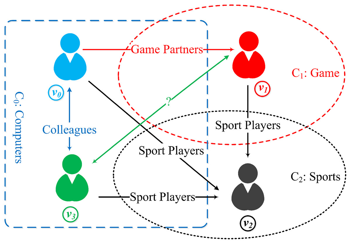
Figure 1: Node information behavior of multiple topic-based communities ( are topic-based communities, and are nodes, and in the meantime ).
Nodes interact in intra-community, such as nodes . Nodes in different communities may interact with each other, such as nodes and and and . Due to the existence of bridge nodes or , nodes and may have a link which is not represented in the current network.
To tackle the above-identified problems, we make the following contributions: (1) We demonstrate the importance of integrating structure features, attributed features, and node’s information behavior features in attribute networks. (2) We propose a joint embedding framework IBE to add the information behavior feature vector to a basic vector to obtain a final joint embedding vector, which has never been considered in the literature. The basic vector is generated by one of existing embedding methods. Within the framework, we design an algorithm ISR to generate a topic-sensitive vector for a given topic, and then we get information behavior feature vectors by matrix transposing a topic-sensitive embedding matrix composed of all topic-sensitive vectors. (3) We conduct extensive experiments in real-world information networks. Experimental results prove the effectiveness and efficiency of the proposed ISR algorithm and IBE framework.
The rest of the article is organized as follows. “Related Work” discusses several related works. We provide some definitions and problem formulation in “Problem Definition”. “Our Approach” presents in detail our proposed IBE framework and ISR algorithm. We then show experimental results in “Experiments” before concluding the article in “Conclusion and Future Work”.
Related work
In the last few years, a large number of NE models have been proposed to learn node network embedding efficiently. These methods can be classified into two categories based on structural information and attributes: (1) SNE methods by considering purely structural information; and (2) ANE methods by considering both structural information and attributes. In this section, we briefly review related work in these two categories.
SNE methods
DeepWalk (Perozzi, Al-Rfou & Skiena, 2014) employs Skip-Gram (Mikolov et al., 2013) to learn the representations of nodes in the network. It uses a random selection of nodes and truncated random walk to generate random walk sequences of fixed length. Subsequently, these sequences are transported to the Skip-Gram model to learn the distributed node representations. LINE (Tang et al., 2015) studies the problem of embedding very large information networks into low-dimensional vector spaces. Node2vec (Grover & Leskovec, 2016) improves the strategy of random walk and achieves a balance between BFS and DFS. SDNE (Wang, Cui & Zhu, 2016) proposes a semi-supervised deep model, which can learn a highly nonlinear network structure. It combines the advantages of first-order and second-order estimation to represent the global and local structure attributes of the network. Besides, there are many other SNE methods (Goyal & Ferrara, 2017), which systematic analysis of various structural graph embedding models, and explain their differences. Nevertheless, these methods fully utilize structural information but do not consider attribute information.
ANE methods
CANE (Tu et al., 2017) proposed an approach of network embedding considering both node text information of context-free and context-aware. CENE (context-enhanced network embedding) (Sun et al., 2016) regards text content as a special kind of nodes and leverages both structural and textural information to learn network embeddings. TopicVec (Li et al., 2016) proposes to combine the word embedding pattern and document topic model. JMTS (Alam, Ryu & Lee, 2016) proposes a domain-independent topic sentiment model to integrate topic semantic information into embedding. ASNE (Liao et al., 2018) adopts a deep neural network framework to model the complex interrelations between structural information and attributes. It learns node representations from social network data by leveraging both structural and attribute information. ABRW (Hou, He & Tang, 2018) reconstructs a unified denser network by fusing structural information and attributes for information enhancement. It employs weighted random walks based network embedding method for learning node embedding and addresses the challenges of embedding incomplete attributed networks. AM-GCN (Wang et al., 2020) is able to fuse topological structures, and node features adaptively. Moreover, there exist quite a few survey papers (Jiao et al., 2021; Zhang et al., 2020; Daokun et al., 2017; Peng et al., 2017; Cui et al., 2019), which provide a comprehensive, up-to-date review of the state-of-the-art network representation learning techniques. They cover not only early work on preserving network structure, but also a new surge of incorporating node content and node labels.
It is challenging to get network embedding considering attributes of local context and topic due to its complexity. Quite a few works have been carried out on this issue. However none of them consider node information behavior features in attributed networks.
Problem definition
In this section, we present the necessary definitions and formulate the problem of link prediction in attributed networks.
Definition 1 (Networks) A network can be represented graphically: G = (V, E, , A), where represents the set of nodes, and |V| is the total number of nodes in G. is the set of edges between the nodes. is a set, where represents a topic and it is also a topic-based node label identified the topic of the node, τ is the total number of topics. A is a function which associates each node in the network with a set of attributes, denoted as A(v).
Definition 2 (Adjacent-Node and Node degree) An adjacent-node set of node v ∈ V is defined as . vdegree is the number of nodes in the adjacent-node set of v, called the degree of node v.
Definition 3 (Topic-based community) Each node v has topic-based labels to identify the topics it belongs to. A topic-based community is a node-set that consists of the nodes with same topic-based label. Here, we define a topic-based community as , and the node number in Cδ is defined as |Cδ|. The topic-based community set is represented as ( = V), where is a set of all topic-based communities. Note that we assume that each node has at least one topic-based label, and one node can belong to several topic-based communities.
Definition 4 (Information behavior) Information behavior is an individual node’s action in a topic category, including information inquiry, information access, information interaction, information sharing, etc.
A message passing is a process of global information recursive, such as GCN. Different from the mechanism of message passing, the information behavior is a process of local-independent information aggregation.
Definition 5 (Importance Score) Given a topic δ, the importance score xi (0 ≤ i < |V|) of node vi is computed as follows:
(1) where 0 ≤ β ≤ 1 is a hyper-parameter, mi and si are the adjacent score and community score of node vi, respectively. vi’s adjacent score mi is defined as the weighted importance score of its adjacent nodes:
where xk is the importance score of vk, is the degree of node vk, and Ni is the adjacent-node set of node vi. Moreover, vi’s community score si with respect to the topic δ is defined as:
where Cδ is a topic-based community and |Cδ| is the number of nodes in Cδ.
The importance score xi of node vi reflects the interaction between vi and its adjacent nodes Ni, as well as the level of correlation between vi and its topic-based community Cδ (δ ∈ Δ).
Definition 6 (Topic-sensitive vector) Given a topic δ, the importance scores of all nodes can be used to form a topic-sensitive vector = .
The learning process of the topic-sensitive vector is a repetitive iteration process for computing the importance scores of all nodes. The initial importance scores is (β = 0.85 is a hyper-parameter; si = if vi ∈ Cδ, otherwise si = 0.). Illustrated by Eq. (1), each iteration is an one-order aggregate operation of adjacent scores and community score and a new value is added to xi for node vi. After a number of iterations (i.e., higher-order aggregations), the ratio between xi of each node vi will stabilize, but the xi for each node vi will continue to grow due to the continuous addition of the vi’s community score si. So, after each iteration, we normalise the xi for every node by
In this way, the xi obtained from this iteration process will eventually converge.
Attributed network embedding. Given an attributed network G = (V, E, Δ, A), our goal is to extract the node information behavior features and learn an information behavior feature vector (d = K * τ, ) for each node v. The distance between and is the information behavior similarity of two nodes v, v′ (v, v′ ∈ V). After that, node information behavior feature vector is added to the node basic vector (d′ |V|) generated by one of existing embedding methods to get the ultimate joint embedding vector:
(2) where [·||·] denotes concatenating two vectors end to end. Nodes with similar network-structure features, node-attribute features, and information-behavior features are close to each other in the embedding space .
Our approach
In this section, we introduce our method of information behavior features extraction. We firstly propose our framework IBE (Information behavior extraction framework) which elaborates the components of node joint embedding vectors. Then, we present the model TNE (Topic-sensitive network embedding model) which describes the process of generating information behavior feature vectors.
Information behavior extraction framework (IBE)
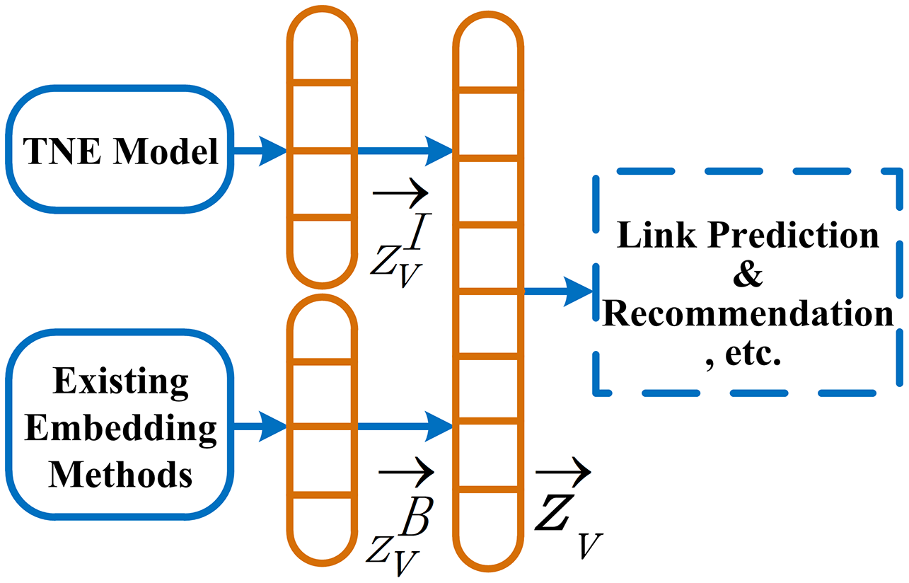
The information behavior features generated based on topics are complementary to features of existing models. As shown in Fig. 2, data sources of the framework IBE consist of two parts. One is the network embedding ZB generated by one of existing embedding methods, and the other is ZI, where and (d′, d ≪ |V|) are embedding matrix consisting of the embedding vectors and of nodes V, respectively. We linearly concatenate the embedding matrix ZB and ZI to generate a joint embedding matrix Z, which can be used for link prediction, recommendation, and other tasks in attributed networks.
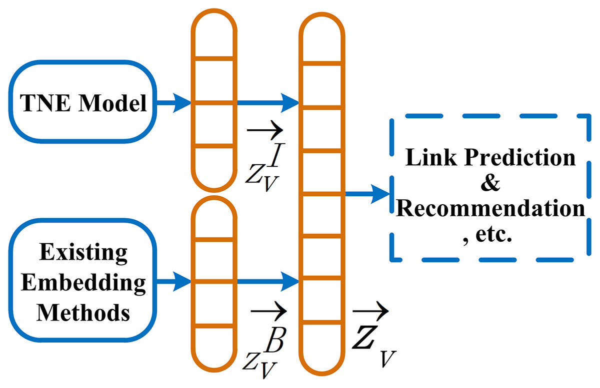
Figure 2: Our information behavior extraction framework (IBE).
Topic-sensitive network embedding model (TNE)
In this section, we present the process of extracting node information behavior features. As shown in Fig. 3, the TNE model consists of two parts: an ISR algorithm (Importance score rating algorithm) and a topic-sensitive embedding matrix (Γ) transposing.
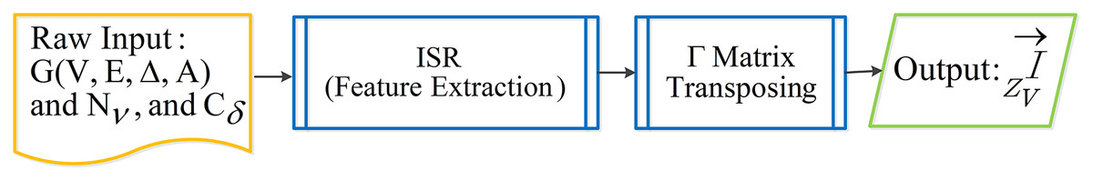
Figure 3: Overview of TNE model.
Importance score rating algorithm (ISR)
The ISR algorithm is used to get the importance scores of all nodes (illustrated by Eq. (1) and Definition 5) and generates a topic-sensitive vector under a given topic. We firstly input raw data including a node set V, an adjacent-node set Nv, and a topic-based community Cδ to ISR (see Algorithm 1) and then simulate the iteration process of node information behavior under the given topic δ. When the importance scores of all nodes stabilize, the iteration is terminated. We propose loss as a metric for iteration termination, which is calculated as follows.
| Input: δ: a topic, δ ∈ Δ; |
| V: a node set of network G; |
| |V|: node number of network G; |
| Ni: a adjacent node set of node vi; |
| videgree: degree of node vi ∈ V; |
| Cδ: a topic-based community, Cδ ∈ CΔ; |
| |Cδ|: node number of topic-based community δ; |
| β = 0.85: a hyper-parameter, imposing the ratio between mi and si; |
| Output: γδ; |
| 1 , initializing every element of list γδ and with in a given topic δ ∈ Δ, where is used to temporarily store a topic sensitive vector; |
| 2 loss = 30; |
| 3 while do |
| 4 loss = 0; norm = 0; |
| 5 for each vi ∈ V do |
| 6 for each vk ∈ Ni do |
| 7 xk = γδ[vk]; mi = mi + ; |
| 8 end |
| 9 if vi ∈ Cδ then |
| 10 si = ; |
| 11 else |
| 12 si = 0; |
| 13 end |
| 14 xi = β * mi + (1 − β) * si; γδ[vi] = xi; norm = norm + ; |
| 15 end |
| 16 norm = ; |
| 17 for each vi ∈ V do |
| 18 γδ[vi] = ; loss = loss + (|γδ[vi] − ); ; |
| 19 end |
| 20 end |
| 21 return γδ = [x0, x1, …, x(|V|−1)]; |
(3) where xi is the current iterative importance score for the node vi and xi′ is the importance score of the previous iteration for the node vi.
After the iteration is done, we can obtain a |V|-dimensional topic-sensitive vector = (x0, x1, …, x(|V|−1)) (illustrated by Definition 6), consisting of importance scores of all nodes under a given topic δ ∈ Δ.
Given a topic δ, the computing steps of topic-sensitive vector are given as follows (see Algorithm 1):
For a node vi, the line 6–8 is used to compute its adjacent scores mi of all of neighbors Ni and the line 9–13 are used to compute its community score si. Using mi and si, the importance scores xi of node vi is finally calculated out in the first statement of line 14.
The second layer loop (line 5, line 14–15) is used to assemble the importance scores of all nodes to generate a list γδ = [x0, x1, …, x(|V|−1)] in program which is the topic-sensitive vector = (x0, x1, …, x(|V|−1)) .
The third statement of line 14 and line 16 are use to calculate the Euclidean norm norm. The line 17–19 is used to normalise the importance scores of all nodes by the Euclidean norm (the first statement of line 18) and calculate the sum of loss for all node (the second statement of line 18). The third statement of line 18 is used to update the value of node vi, which is the importance score and will be used in the next iteration.
The first layer loop (line 3, line 20) is used to control the iterations.
In the ISR algorithm, an information behavior feature vector is generated without an increase in time complexity. We define L as the number of iterations, n represents the number of nodes in attributed networks, and vdegree represents the degree of node v. The time complexity of the ISR algorithm to generate a topic-sensitive vector = (x0, x1, …, x(|V|−1)) is . Because L · vdegree and n are of the same order of magnitude, the time complexity of the ISR algorithm is thus .
Topic-sensitive embedding matrix (Γ) transposing
For Δ = {δ0, δ1, …, δ(τ−1)}, the Γ matrix transposing calls the Algorithm 1 to get every topic-sensitive vectors in each topic δ ∈ Δ. After all τ topic-sensitive vectors are obtained, we combine the τ topic-sensitive vectors to form a topic-sensitive embedding matrix Γ = , , …, . Ultimately, ZI is obtained by the Γ matrix transposing, as illustrated by Eq. (4).
(4)
Each row of ZI is an information behavior feature vector for node v and the dimension of is d = τ.
Generating node joint embedding vectors based on IBE
ZB is a basic embedding matrix trained by one of existing embedding methods. Each row of the ZB is a basic vector for a node v generated by one of existing embedding methods.
Before getting Z by Eq. (7) according to the framework IBE, we firstly enlarge ZI or ZB by λ (Eq. (5)) so that the element values of λ * ZI and ZB or ZI and are of the same order of magnitude, and the λ is calculated as follows.
(5) where is the average of all elements in ZB, and is the average of all elements in ZI. And then we enlarge the element values of ZI or ZB who has the larger AUC (Hanley & Mcneil, 1982) value by weight coefficient α (Eq. (6)) again.
(6) where auc() is a function used to calculate the value of AUC, ψ is an amplification factor of the ratio .
Especially, we should not use the method of reducing the element values of ZI or ZB to make their element values of the same order of magnitude, because it may result in invalid results due to the element values are too small. So, according to the values of coefficients α and λ, we divide the methods of linearly concatenating ZI and ZB into four cases as follows.
(7) where the operator [·||·] denotes concatenation, α is an enlarging coefficient to make the joint embedding matrix Z more similar to ZI or ZB who has the higher AUC value, and λ (Eq. (5)) denotes the enlargement factor who try to be adjusted to make the element values of λ * ZI and ZB or ZI and in the same order of magnitude.
For the case of [(α * λ * ZI) ‖ ZB] (λ ≥ 1 and α ≥ 1) in Eq. (7), Z is displayed in matrix form as follows:
where each row of Z is the final joint embedding vector for node v based on the framework of IBE and xij (0 ≤ i < |V|, 0 ≤ j < τ) is the element of , bij (0 ≤ j < d) is the element of . The other three cases of Eq. (7) have similar matrix representations.
Experiments
In this section, we describe our datasets, baseline models and present the experimental results to demonstrate the performance of the IBE framework in link prediction tasks. The source code and datasets can be obtained from https://github.com/swurise/IBE.
Datasets
In Table 1, we consider the following real-world network datasets. BlogCatalog (http://networkrepository.com/soc-BlogCatalog.php) is asocial blog directory. The dataset contains 39 topic labels, 10,312 users, and 667,966 links. Zhihu is the largest online Q & A website in China. Users follow each other and answer questions on this site. We randomly crawl 10,000 active users from Zhihu and take the descriptions of their concerned topics as text information (Tu et al., 2017). The topics of Zhihu are obtained by the fastText model (Joulin et al., 2016) and the ODP of predefined topic categories (Haveliwala, 2002). The fastText presents the hierarchical softmax based on the Huffman tree to improve the softmax classifier taking advantage of the fact that classification is unbalanced in CBOW (Joulin et al., 2016). WiKi contains 2,408 documents from 17 classes and 17,981 edges between them. Cora is a research paper classification citation network constructed by McCallum et al. (2000). After filtering out papers without text information, 2,277 machine learning papers are divided into seven categories and 36 subcategories in this network. Citeseer is divided into six communities: Agents, AI, DB, IR, ML, and HCI and 4,732 edges between them. Similar to Cora, it records the citing and cited information between papers.
| Dataset Name | Social network | Language network | Citation network | ||
|---|---|---|---|---|---|
| BlogCatalog | Zhihu | Wiki | Cora | Citeseer | |
| Nodes | 10,312 | 10,000 | 2,408 | 2,277 | 3,312 |
| Edges | 667,966 | 43,894 | 17,981 | 5,214 | 4,732 |
| Attributes | – | 10,000 | – | 2,277 | – |
| Number of topics (τ) | 39 | 13 | 17 | 7 | 6 |
Baselines
To validate the performance of our approach, we employ several state-of-the-art network embedding methods as baselines to compare with our IBE framework. A number of existing embedding methods are introduced as follows.
CANE (Tu et al., 2017) learns context-aware embeddings with mutual attention mechanism for nodes, and the semantic relationship features are extracted between nodes. It jointly leverages network structure and textural information by regarding text content as a special kind of node.
DeepWalk (Perozzi, Al-Rfou & Skiena, 2014) transforms a graph structure into a sample set of linear sequences consisting of nodes using uniform sampling. These linear sequences are transported to the Skip-Gram model to learn the distributed node embeddings.
HOPE (Ou et al., 2016) is a graph embedding algorithm, which is scalable to preserve high-order proximities of large scale graphs and capable of capturing the asymmetric transitivity.
LAP (Belkin & Niyogi, 2001) is a geometrically motivated algorithm for constructing a representation for data sampled from a low dimensional manifold embedded in a higher dimensional space.
LINE (Tang et al., 2015) learns node embeddings in large-scale networks using first-order and second-order proximity between the nodes.
Node2vec (Grover & Leskovec, 2016) has the same idea as DeepWalk using random walk sampling to get the combinational sequences of node context, and then the network embeddings of nodes are obtained by using the method of word2vec.
GCN (Kipf & Welling, 2016) model uses an efficient layer-wise propagation rule based on a localized first-order approximation of spectral graph convolutions. The GCN model is capable of encoding graph structure and node features in a scalable approach for semi-supervised learning.
GAT (Veličković et al., 2018) is a convolution-style neural network that operates on graph-structured data, leveraging masked self-attentional layers to address the shortcomings of methods based on graph convolutions. GAT enables implicitly specifying different weights to different nodes within a neighborhood.
Evaluation metrics and parameter settings
We randomly divide all edges into two sets, training set and testing set, and take a standard evaluation metric AUC scores (area under the ROC curve) (Hanley & Mcneil, 1982) as evaluation metrics to measure the link prediction performance. AUC represents the probability that nodes in a random unobserved link are more similar than those in a random nonexistent link. Because the number of topics is different in each dataset, we use τ to denote the maximum number of topics for each dataset. In concatenating weight coefficient α = [auc(ZI) ÷ auc(ZB)]ψ, we set the factor ψ equal to 4 except that ψ has a specified value.
Experimental results
For experiments, we evaluate the effectiveness and efficiency of our IBE on five networks for the link prediction task. For each dataset, we compare the AUC data of basic embedding matrix ZB generating by one of the existing embedding methods, the information behavior feature vectors ZI, and their joint embedding vectors Z generating by the framework IBE. We employ six state-of-the-art embedding methods as baselines, including Node2vec, DeepWalk, LINE, LAP, CANE, HOPE, for comparisons with their extending frameworks IBE in the following experiments.
Table 2 compares AUCs over five datasets. By concatenating ZB and ZI linearly, the joint embedding vectors Z achieves the best performance. Especially on the BlogCatalog and Zhihu datasets, the AUC values of the joint embedding vectors Z are higher, compared with their baselines, than 14.6% and 27.6% respectively on average. One of the reasons may be that the average AUC of information behavior feature vectors ZI are 81.7 and 82.4 respectively, which are more than 11% higher compared with the other three datasets on average. The other reason is that the maximum topic number τ of BlogCatalog and Zhihu are larger than those of Cora and Citeseer. In Table 2, we can also see that most of the AUC values of the joint embedding vectors Z for datasets Wiki and Cora exceed 90%. The reason is that their AUC values of baselines are relatively high, most of them are more than 85%. On the Citeseer dataset of Table 2, we also can see that the improvement of the AUC values of the joint embedding vectors Z is less, compared with their baselines. The result can be explained by the fact that the AUC values of information behavior feature vectors ZI are all low, about 55% and the direct reason for the low AUC values is that the number of topics is too small. Due to the number of topics is small, the topic subdivision degree of nodes is low, and the classification of node labels will not be too detailed.
| Dataset Embedding | Social network | Language network | Citation network | ||
|---|---|---|---|---|---|
| BlogCatalog (τ = 39) | Zhihu (τ = 13) | Wiki (τ = 17) | Cora (τ = 7) | Citeseer (τ = 6) | |
| ZI | 81.5 | 81.5 | 69.1 | 69.9 | 54.5 |
| ZB (CANE) | – | 71.2 | – | 94.5 | – |
| Z (CANE) | – | 85.6 | – | 94.7 | – |
| ZB (DeepWalk) | 72.1 | 58.2 | 90.6 | 89.5 | 84.5 |
| Z (DeepWalk) | 85.0 | 84.9 | 93.5 | 89.5 (ψ = 1) | 85.7 |
| ZB (HOPE) | 83.3 | 64.3 | 92.6 | 84.6 | 70.2 |
| Z (HOPE) | 83.0 | 82.0 (ψ = 6) | 92.7 | 86.7 | 71.2 |
| ZB (LAP) | 75.2 | 74.2 | 92.2 | 87.9 | 80.3 |
| Z (LAP) | 87.3 | 86.0 | 93.2 | 89.1 | 81.5 |
| ZB (LINE) | 59.1 | 51.6 | 87.8 | 78.3 | 69.8 |
| Z (LINE) | 82.1 | 82.8 | 88.1 (ψ = 7) | 80.7 | 73.8 |
| ZB (Node2vec) | 71.0 | 56.1 | 89.0 | 86.7 | 83.2 |
| Z (Node2vec) | 85.2 | 84.5 (ψ = 6) | 93.1 | 88.1 | 84.5 (ψ = 2) |
| ZB (GCN) | – | – | – | 90.2 | 89.7 |
| Z (GCN) | – | – | – | 93.4 | 91.8 |
| ZB (GAT) | – | – | – | 92.6 | 90.2 |
| Z (GAT) | – | – | – | 94.5 | 91.7 |
In general, in Table 2, it can be seen that the AUC values of concatenating embedding vectors Z are higher than that of ZB and ZI, which indicates that the concatenating method can properly integrate the features of all parties.
Ablation experiments: To investigate the effectiveness of TNE, we perform several ablation studies. In Table 2, the ZB is the basic embedding generated by an existing model. The ZI is obtained by the TNE model. A joint embedding Z is obtained by adding a ZI to a ZB, shown in Fig. 2 and Eq. (2). We observe that the quality of the joint embedding Z is better than itself ZB.
Parameter sensitivity analysis
We further performed parameter sensitivity analysis in this section, and the results are summarized in Figs. 4 and 5. Due to space limitations, we only take the dataset of Wiki, Zhihu as an examples to estimate the topic number j (0 ≤ j ≤ τ) and the amplification factor ψ of vector concatenation can affect the link prediction results.
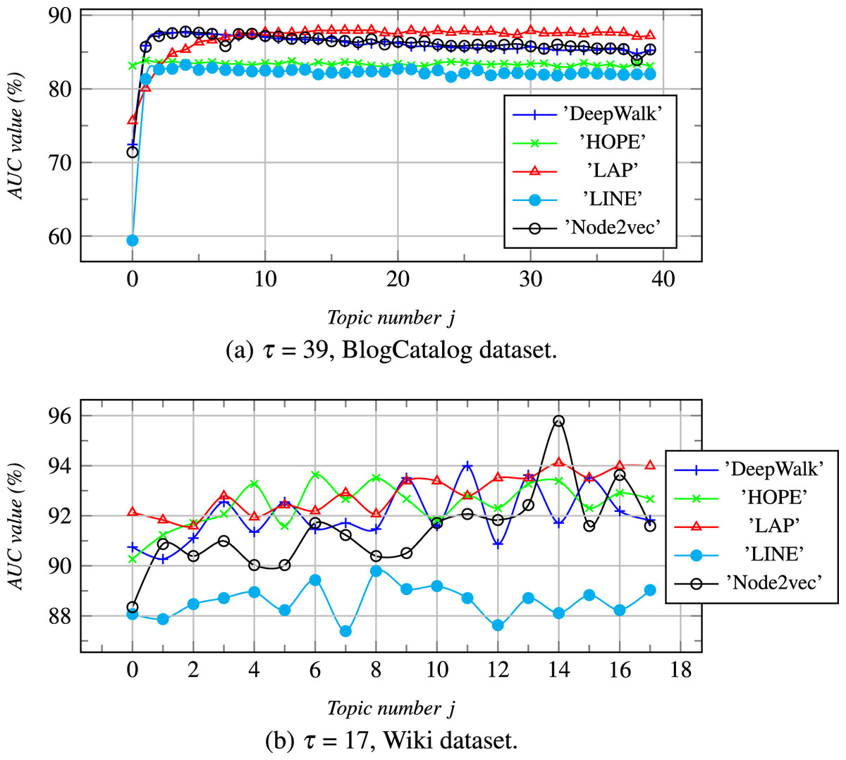
Figure 4: ψ = 5.
With the increase of τ, the AUC values are calculuated for different datasets. j is a topic number, if j = 0 then Z = ZB else Z = [ZB ZI].
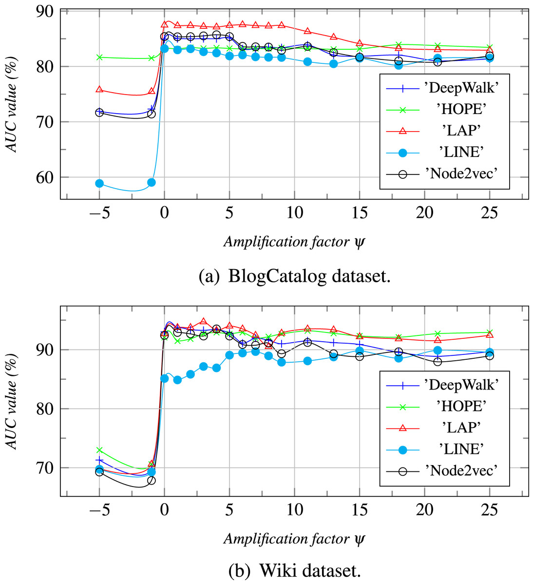
Figure 5: The topic number is τ, and ψ is an amplification factor.
With the increase of ψ, the AUC values are calculated for different datasets.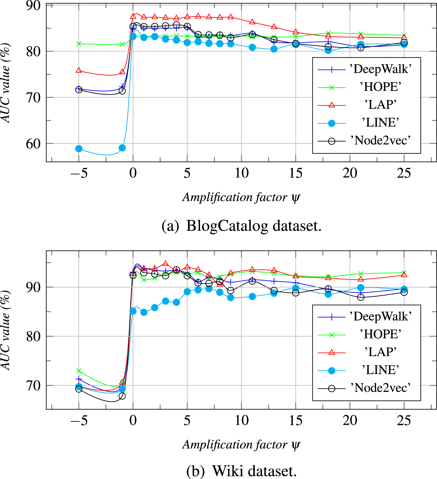
The topic number j (0 ≤ j ≤ τ): In Fig. 4, we illustrate the relationship between the number of topics and link prediction, where the order of selection of node topics is random. When j = 0, ZI does not exist, Z degenerates to ZB. As shown in Fig. 4, we can see that as j increases from 1 to τ, ZB linearly combines with more topic-based feature dimensionality from ZI, and the AUC values keep changing. When the AUC values of ZB are below 82% in Fig. 4A, AUC values increase sharply with an increase of j. When the AUC values of ZB are higher than a certain critical value, the AUC values increase more slowly or even stop growing with an increase of j.
So, we can see that when the number of topics is large in a dataset, each node can be classified in detail by the topic classification labels, which helps to improve the AUC values using a small number of topics. These also show that the AUC values of the concatenating embedding vectors Zs will be higher than that of all parties for concatenating, that is ZIs and ZBs, but it will not increase indefinitely.
The amplification factor ψ of vector concatenation: ψ is an amplification factor for α (Eq. (6)) which is a weight coefficient for enlarging the element values of ZI or ZB who has the larger AUC (Eq. (7)). From Fig. 5, we can see that the AUC value, when ψ is less than 0, is less than that when ψ is greater than 0. The reason is that the weight coefficient α, when ψ is less than 0, enlarges the ZI or the ZB who has the smaller AUC value. As a result, the joint embedding Z is more similar to one that has a lower AUC value. When ψ is between 1 and 5, the prediction result is the best. However, when the value of ψ increases gradually, the AUC values decrease slightly and tend to the ZIs or the ZBs who have the larger AUC values.
Conclusion and future work
This article has presented an effective network embedding framework IBE, which can easily incorporate topology features, attribute features, and features of topic-based information behavior into network embedding. In IBE, we linearly combinate ZI and ZB to generate node joint embedding matrix Z. To get the ZI, we have proposed the TNE model to extract the node’s information behavior features. The model contains an ISR algorithm to generate the topic-sensitive embedding matrix (Γ) and a Γ matrix transposing algorithm to transpose Γ matrix into the information behavior feature matrix ZI for nodes eventually. Experimental results in various real-world networks have shown the efficiency and effectiveness of joint embedding vectors in link prediction. In the future, we plan to investigate other methods of extracting features that may better integrate with the TNE model. Moreover, we will further investigate how the TNE model works in heterogeneous information networks.