
Applying SARIMA, ETS, and hybrid models for prediction of tuberculosis incidence rate in Taiwan
- Published
- Accepted
- Received
- Academic Editor
- Nancy Keller
- Subject Areas
- Epidemiology, Infectious Diseases, Public Health, Respiratory Medicine
- Keywords
- TB incidence, SARIMA, SARIMA-ETS
- Copyright
- © 2022 Kuan
- Licence
- This is an open access article distributed under the terms of the Creative Commons Attribution License, which permits using, remixing, and building upon the work non-commercially, as long as it is properly attributed. For attribution, the original author(s), title, publication source (PeerJ) and either DOI or URL of the article must be cited.
- Cite this article
- 2022. Applying SARIMA, ETS, and hybrid models for prediction of tuberculosis incidence rate in Taiwan. PeerJ 10:e13117 https://doi.org/10.7717/peerj.13117
Abstract
Background
Tuberculosis (TB) remained one of the world’s most deadly chronic communicable diseases. Future TB incidence prediction is a benefit for intervention options and resource-allocation planning. We aimed to develop rapid univariate prediction models for epidemics forecasting employment.
Methods
The surveillance data regarding Taiwan monthly TB incidence rates which from January 2005 to June 2017 were utilized for simulation modelling and from July 2017 to December 2020 for model validation. The modeling approaches including the Seasonal Autoregressive Integrated Moving Average (SARIMA), the Exponential Smoothing (ETS), and SARIMA-ETS hybrid algorithms were constructed and compared. The modeling performance of in-sample simulating training sets and pseudo-out-of-sample validating sets were evaluated by metrics of the root mean square error (RMSE), mean absolute percentage error (MAPE), mean absolute error (MAE), and mean absolute scaled error (MASE).
Results
A total of 191,526 TB cases with a highest incidence rate in 2005 (72.5 per 100,000 person-year) and lowest in 2020 (33.2 per 100,000 person-year), from January-2005 to December-2020 showed a seasonality and steadily declining trend in Taiwan. The monthly incidence rates data were utilized to formulate these forecasting models. Through stepwise screening and assessing of the accuracy metrics, the optimized SARIMA(3,0,0)(2,1,0)12, ETS(A,A,A) and SARIMA-ETS-hybrid models were respectively selected as the candidate models. Regarding the outcome assessment of model performance, the SARIMA-ETS-hybrid model outperformed the ARIMA and ETS in the short term prediction with metrics of RMSE, MAE MAPE, and MASE of 0.084%, 0.067%, 0.646%, and 0.870%, during the pseudo-out-of-sample forecasting period. After projecting ahead to the long term forecasting TB incidence rates, ETS model showed the best performance resulting as a 41.69% (range: 22.1–56.38%) reduction of TB epidemics in 2025 and a 54.48% (range: 33.7–68.7%) reduction in 2030 compared with the 2015 levels.
Conclusion
This time series modeling might offer us a rapid surveillance tool for facilitating WHO’s future TB elimination milestone. Our proposed SARIMA-ETS or ETS model outperformed the SARIMA in predicting less or 12–30 months ahead of epidemics, and all models showed better in short or medium-term forecasting than long-term forecasting.
Introduction
Tuberculosis (TB) is a chronic respiratory infection caused by the Mycobacterium tuberculosis complex, most commonly transmitted by cough aerosols (World Health Organization (WHO), 2018; Turner & Bothamley, 2015). Despite efforts to combat this devastating disease, tuberculosis remains a major global health problem due to high morbidity, medical costs, drug resistance, and coinfection, creating a huge health burden (World Health Organization (WHO), 2018; Turner & Bothamley, 2015; Stewart, Robertson & Young, 2003). Although the global TB incidence has declined by 1–2% per year, it is still a major public health problem, with an estimated 1.3 million new infections and 1.8 million deaths from tuberculosis worldwide in 2018 (World Health Organization (WHO), 2018). Taiwan is a median tuberculosis country with incidence.
The World Health Organization proposed the End TB Strategy in 2014, intending to reduce TB deaths by 90% and mitigate incident cases by 80% between 2016 and 2030 (Floyd et al., 2018; Floyd et al., 2018). To achieve this ambitious goal, disease trend prediction is of great benefit for options of future control interventions and allocations of the health resources. Instead, other than using multivariate factors to establish prediction models, many literatures also had deliberate the need of prediction models by a univariate time series analysis, especially in quickly planning the future resource allocation. One of the widely applied time series analysis modeling tool is the autoregressive integrated moving average (ARIMA) model, a widely applied time series analysis tool, proposed by George Box and Gwilym Jenkins in the 1970s (Coulombier, Quenel & Epiet, 2004). ARIMA was widely applied in communicable disease predictions such as malaria, hemorrhagic fever, hand-foot-mouth disease, influenza, COVID19, and tuberculosis (Liu et al., 2020; Wang et al., 2018; Benvenuto et al., 2020). Additionally, ARIMA-related hybrid models such as SARIMA-ETS-hybrid models were also developed as modeling candidates for future trend prediction (Benvenuto et al., 2020; Mohammed et al., 2018).
In this study, we applied the time series analysis approach to construct optimized univariate forecasting models for tuberculosis incidence rapid forecasting in Taiwan. The seasonal automatic autoregressive integrated moving average (SARIMA), exponential smoothing state space (ETS) and the SARIMA-exponential smoothing state space (ETS)-hybrid models would be constructed to interpret the historical tuberculosis incidence trends and seasonality. Also, the accuracy of simulating performance as well as future predicting algorithms for epidemic warnings of the near future and toward far facilitation plans for WHO’s TB control goal would be assessed.
Materials and Methods
Data source
Data of the TB cases and population were obtained respectively from the websites of the Taiwan Center for Disease Control (CDC) (Taiwan National Infectious Disease Statistics System, https://nidss.cdc.gov.tw/ch/SingleDisease.aspx?dc=1&dt=3&disease=010) and the Taiwan Ministry of the Interior (Ministry of Interior Taiwan. Statistics: annual report of the Ministry of the Interior, Table S2). Then, the TB morbidity was subsequently calculated. All TB cases were initially diagnosed by clinical symptoms as well as confirmed by bacteriological and pathological examinations. In Taiwan, TB is a nationally notifiable disease, and hospital physicians must report cases promptly, i.e., cases of TB must be registered within 7 days, via the Taiwan TB registry system authorized by the Taiwan CDC for national-level surveillance purposes (Taiwan Centers for Disease Control, Department of Health. Taiwan Tuberculosis Control Report, https://www.cdc.gov.tw/En/InfectionReport/List/SOIzsdQ5fRn3xPZOleIb0w).
The study period included cases diagnosed from 2005 January to 2020 December, and TB incidence data set (Annex A: Availability of raw data) was aggregated and analyzed monthly based on the public data from confirmed cases. The data were divided into training data and validation datasets. Then, respectively, generated simulating models based on the data from 2005 January to 2017 June (in-sample, training dataset). And, the forecasting testing model was based on the data from 2017 July to 2020 December (pseudo-out-of-sample, forecast test dataset). Thereafter, we utilized the optimizing models to project the future prediction toward 2025 December.
STL decomposition
The Seasonal and Trend decomposition using Loess analysis was adopted for decomposing time series into trend, seasonal, and remainder components which developed by Cleveland, Cleveland & McRae (1990).
Construct of the SARIMA and SARIMA-ETS hybrid model
SARIMA model
The seasonal autoregressive integrated moving average (SARIMA) model is a Seasonal ARIMA (Coulombier, Quenel & Epiet, 2004; Liu et al., 2020; Wang et al., 2018; Benvenuto et al., 2020; Mohammed et al., 2018). The general form of the SARIMA model is as follows: (p,d,q)(P,D,Q)S, where p and q are the orders of the autoregressive (AR) and moving average (MA) components, respectively, d is the order of the differences, P, D and Q are the corresponding seasonal orders, and S represents the steps of the seasonal differences. The SARIMA model was established based on the rationale as the previous description. We constructed it by auto.arima function in R package. The best performing model was automatically chosen according to the minimum AIC (Aho, Derryberry & Peterson, 2014), AICc or BIC (Aho, Derryberry & Peterson, 2014).
ETS model
The ETS model considers the error, trend, and seasonal components of a given time series and evaluates possible alternative models before selecting the best-performing model to simulate the data (Ministry of Interior Taiwan. Statistics: annual report of the Ministry of the Interior, https://www.moi.gov.tw/files/site_stuff/321/1/month/month_en.html). The major three parameters are the error, trend, and seasonal components, which can be additive (A), multiplicative (M), or none (N). It was constructed by the ETS function in the R package. As a forecasting model incorporating the foundations of exponential smoothing, the ETS technique provided the forecast package for the R software outlined by Hyndman. The best performing model was automatically chosen according to the minimum AIC (Aho, Derryberry & Peterson, 2014), AICc or BIC (Aho, Derryberry & Peterson, 2014). As automatic forecasting models incorporating the foundations of the ETS techniques were provided in the R software package outlined by Hyndman (Hyndman, Koehler & Snyder, 2002). The Ljung-Box Q test was also used to diagnose whether the residual error sequence was a white-noise sequence.
Ensemble model
Hybrid forecast model comprised of the following models of equal weight i.e., with 0.5 weight ARIMA model and 0.5 weight ETS model. As automatic forecasting models incorporating the foundations of SARIMA-ETS-hybrid techniques were provided in the R software package developed by Shaub and Ellis (Shaub & Ellis, 2020).
Evaluation metrics
To evaluate the performance of the SARIMA, ETS or SARIMA-ETS models, the fitted values were tested. Several performance measures were employed in determining the prediction efficiency of the automatic ARIMA model, namely, the Akaike information criterion (AIC) (Aho, Derryberry & Peterson, 2014), root means square error (RMSE) (Woschnagg, 2004), mean absolute error (MAE) (Woschnagg, 2004), mean absolute percentage error (MAPE) (Woschnagg, 2004) and the mean absolute scaled error (MASE) (Woschnagg, 2004; Hyndman, 2006). These metrics have been used by many researchers to evaluate accuracy. For these metrics, the smallest values correspond to the optimal methods.
Software
We applied the time-series model, the forecast and related packages in R (version 4.0.1). The used functions and hyperparameters were listed in Table 1.
| No | Series | Model | Estimated parameter | AICc/Accuracy | Residuals check (Ljung-Box test dat) |
|---|---|---|---|---|---|
| 1 | Training set of TB incidence (150 observations) | ARIMA(1,0,0)(2,1,0) by R, package: forecast, function: auto.arima | Coefficients: ar1 = −0.2399, sar1 = −0.6395, sar2 = −0.2443, drift = −0.0038 s.e. 0.0866 0.0882 0.0907 0.0002 sigma^2 estimated as 0.00475: log likelihood = 172.81 |
AIC = −335.62, AICc = −335.17, BIC = −320.99; RMSE = 0.0652 MAPE = 0.5127 |
Residuals from ARIMA(1,0,0)(2,1,0) with drift, Q* = 62.283, df = 20, p-value = 3.139e−06, Model df: 4. Total lags used: 24 |
| 2 | Simulation set of TB incidence (192 observations) | ARIMA(3,0,0)(2,1,0) by R, package: forecast, function: auto.arima | Coefficients: ar1 = 0.1283, ar2 = 0.1111, ar3 = 0.2527, sar1 = −0.6137, sar2 = −0.3464, drift = −0.0041 sigma^2 estimated as 0.005094: log likelihood = 219.89 |
AIC = −425.79 AICc = −425.14 BIC = −403.44 RMSE = 0.0652, MAPE = 0.5213 |
Residuals from ARIMA(3,0,0)(2,1,0) with drift Q* = 34.641, df = 18, p-value = 0.01048, Model df: 6. Total lags used: 24 |
| 3 | Training set of TB incidence (150 observations) | ETS(A,A,A) | Smoothing parameters: alpha = 0.0102, beta = 0.0101, gamma = 1e−04; |
AIC = −68.44, AICc = −63.81, BIC = −17.26 RMSE = 0.0581, MAPE = 0.4591 |
Residuals from ETS(A,A,A); Q* = 61.132, df = 8, p-value = 2.793e−10; Model df: 16. Total lags used: 24 |
| 4 | Simulation set of TB incidence (192 observations) | ETS(A,A,A), Call: ets (y = M) |
ETS(A,A,A) Call: ets (y = M) Smoothing parameters: alpha = 0.0738, beta = 1e−04, gamma = 1e−04 , |
AIC = −25.56 AICc = −22.04 BIC = 29.82 RMSE = 0.0618, MAPE = 0.4870 |
Residuals from ETS(A,A,A); Q* = 51.531, df = 8, p-value = 2.073e−08; Model df: 16. Total lags used: 24 |
| 5 | Training set of TB incidence (150 observations) | ARIMA-ETS | Hybrid forecast model comprised of the following models: arima with weight 0.5, ETS with weight 0.5 | RMSE = 0.0585 MAPE = 0.4613 |
Could not find appropriate degrees of freedom for this model |
| 6 | Simulation set of TB incidence (192 observations) | ARIMA-ETS | Hybrid forecast model comprised of the following models: arima with weight 0.5, ETS with weight 0.5 | RMSE = 0.0512 MAPE = 0.5058 |
Could not find appropriate degrees of freedom for this model |
Results
General information and analysis of the time series
There were 191.526 newly confirmed TB cases in Taiwan, with an average monthly incidence rate of 4.392 (range: 2.287–6.937) per 100,000 population per month, during the study period of 192 months, i.e., from January 2005 to December 2020. Through the STL analysis, we isolated seasonality and overall trend components from the monthly TB data series and also eliminated part of the random noise or reminder components. As shown in Fig. 1, the outcome of the seasonal-trend decomposition method, yields an overall trend with several composers including a 12-month stochastic seasonality; a downward overall trend with highest in 2005 (72.5 per 100,000 person-year) and lowest in 2020 (33.2 per 100,000 person-year) as well as a periodically change of disease incidences (Figs. 1A, 1C). Also applied a box plot suggested that there was seasonality in the data. It could be seen obviously that the variation of TB in Taiwan showed the periodicity within 1 year (12 months) being a cycle with obvious seasonality during the variation process in each year with two peaks occurring in March and May as well as a trough from December to February in each cycle (Figs. 1B, 1C).
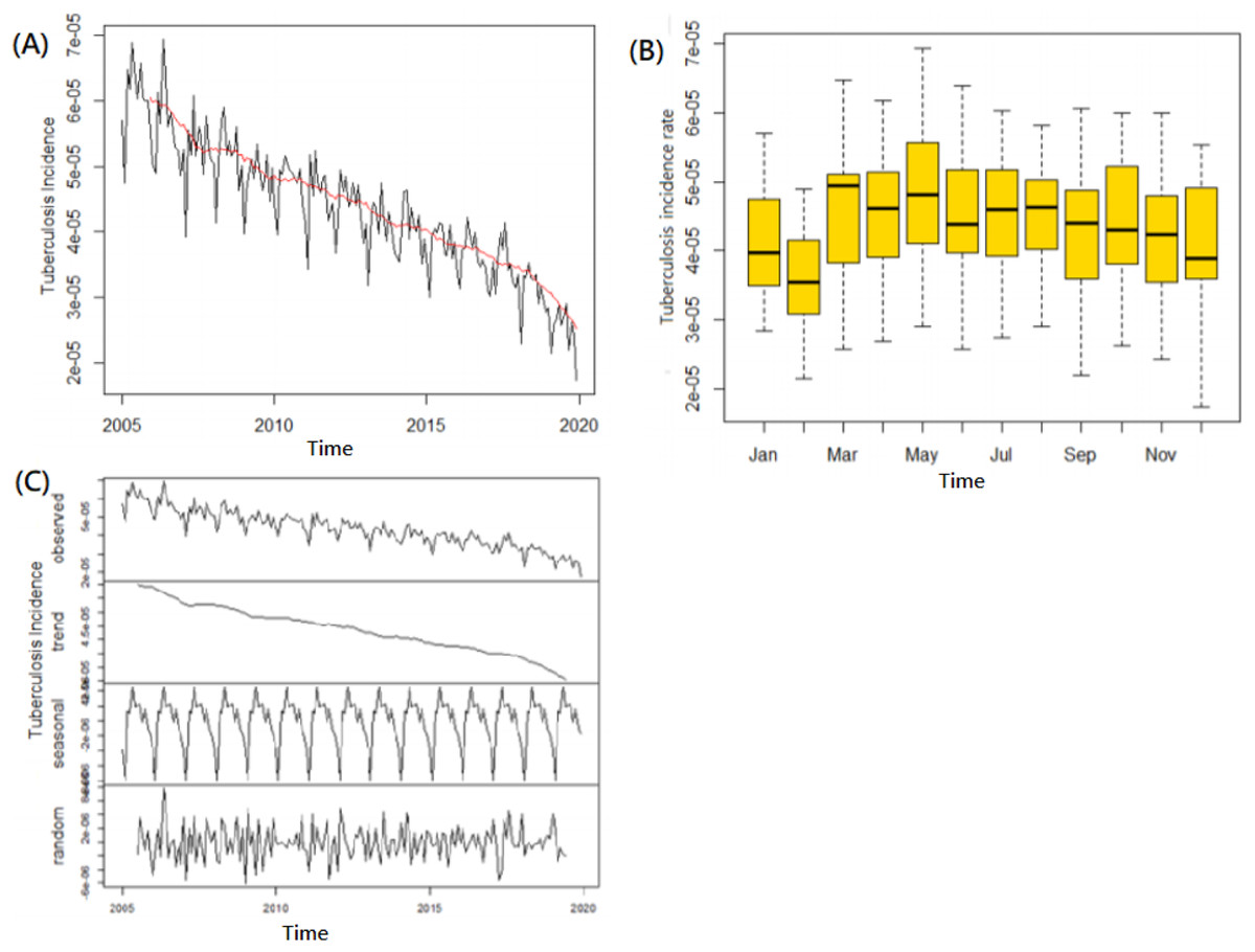
Figure 1: Tuberculosis incidence time series analysis of trend and seasonality.
(A) Tuberculosis incidence with a steady declining trend from 2005–2019. (B) Box-plotting to present a seasonality with two peaks occurring in March and May as well as a trough in November to the next February. (C) STL Decomposition of the time series.
The incidence data set was used to analyze and formulate the simulating models. We applied the time series including 192 datasets of logarithmic monthly incidence rates which counterbalanced by an order of 12 at the seasonal level. The outcome of an Augmented Dickey-Fuller test (Dickey-Fuller = −7.6315, Lag order = 1, PDickey-Full = 0.01 of alternative hypothesis: stationary) and Ljung-Box test (X-squared = 125.87, df = 1, PLjung-box = <2.2e−16 of alternative hypothesis: being not independent) which showed that this time series of from January 2005–December 2020 was with stationary and serial correlation format (Fig. 1A).
Construct and compare the accuracy metrics of modeling performances: simulating training by in-sample sets and evaluate or validate forecasting testing by pseudo out-of-sample sets
For constructing and evaluating the accuracy of the modellings, the simulating processing, and forecasting performances were assessed and verified, respectively. Beforehand, the data series samples were divided into the training sets (in samples) i.e., the former 150 datasets from January 2005 to June 2017, and the forecasting test sets (pseudo-out-of-samples) i.e., the following 42 data series from July 2017 to December 2020. Next, three training models were constructed utilized 150 datasets. Firstly, a best-simulating ARIMA in samples identified the seasonal ARIMA(1,0,0)(2,1,0)12 mode was selected as the best performing ARIMA model with the most minimum values of AIC = −335.62, BIC = −320.99. According to its Ljung-Box Q test which showed the fitness of the ARIMA(1,0,0)(2,1,0)12 models with the residual error, the sequence was achieved white noise of Q* = 62.283, p-value = 3.139e−06. Secondly, a ETS(A,A,A) model (AIC = −68.44, BIC = −17.26) was selected as the best performing ETS model with the Ljung-Box Q testing showed that Q* = 46.357, p-value = 2.033e−07. Thirdly, a hybrid model was constructed and comprised of the following models: ARIMA with a weight 0.5 and ETS with a weight 0.5 (Tables 1, 2).
| Ahead time | Actual-value (cases per 105-month | Models | Prediction (cases per 105-month) | 95% CI of PV | RMSE | MAE | MAPE | MASE |
|---|---|---|---|---|---|---|---|---|
| 3 months 2017-09 |
3.55 | SARIMA(1,0,0)(2,1,0)12 | 3.43 | [2.77–4.14] | 0.086 | 0.058 | 0.575 | 0.753 |
| ETS | 3.49 | [2.93–4.14] | 0.077 | 0.058 | 0.569 | 0.746 | ||
| Hybrid | 3.39 | [2.77–4.13] | 0.081 | 0.056 | 0.554 | 0.726 | ||
| 6 months 2017-12 |
3.3 | SARIMA | 3.34 | [2.76–4.15] | 0.069 | 0.047 | 0.459 | 0.606 |
| ETS | 3.29 | [2.76–3.97] | 0.060 | 0.046 | 0.449 | 0.593 | ||
| Hybrid | 3.4 | [2.79–4.15] | 0.064 | 0.045 | 0.445 | 0.587 | ||
| 12 months 2018-6 |
3.15 | SARIMA | 3.58 | [2.9–4.51] | 0.088 | 0.062 | 0.598 | 0.606 |
| ETS | 3.47 | [2.9–4.14] | 0.079 | 0.061 | 0.586 | 0.785 | ||
| Hybrid | 3.69 | [3.03–4.51] | 0.082 | 0.060 | 0.578 | 0.776 | ||
| 18 months 2018-12 |
3.15 | SARIMA | 3.16 | [2.55–4.0] | 0.090 | 0.069 | 0.668 | 0.898 |
| ETS | 3.09 | [2.55–3.73] | 0.080 | 0.065 | 0.627 | 0.849 | ||
| Hybrid | 3.23 | [2.62–4.0] | 0.084 | 0.066 | 0.639 | 0.859 | ||
| 24 months 2019-6 |
3 | SARIMA | 3.4 | [2.64–4.4] | 0.092 | 0.074 | 0.714 | 0.960 |
| ETS | 3.26 | [2.64–4.02] | 0.079 | 0.065 | 0.627 | 0.812 | ||
| Hybrid | 3.41 | [2.64–4.4] | 0.084 | 0.068 | 0.655 | 0.881 | ||
| 30 months 2019-12 |
3 | SARIMA | 2.89 | [2.38–3.51] | 0.091 | 0.073 | 0.699 | 0.942 |
| ETS | 2.90 | [2.28–3.69] | 0.079 | 0.064 | 0.619 | 0.833 | ||
| Hybrid | 2.98 | [2.28–3.9] | 0.084 | 0.067 | 0.646 | 0.870 |
Notes:
Evaluation of the models’ accuracy of the SARIMA. ETS and SARIMA-ETS hybrid in forecasting underlying trend (pseudo out-of-sample) performance.
Prediction: TB incidence (cases per 100,000-month); Hybrid: SARIMA-ETS-hybrid.
95% CI of PV: 95% confidence interval of predictive value for TB incidence.
Subsequently, the forecasting tests were performed, i.e., a 6-to-30-months ahead forecasting steps were computed. Thus, the modeling’ accuracy metrics were estimated respectively based on these yield forecasting values from the simulating model constructed by the 150 in-sample training datasets. Overall, several metrics were employed to evaluate the performance of these preferred models including their in-sample simulating and out-of-sample forecasting for comparison. Regarding the performance of the simulated fitting, the RMSE, MAE, MAPE and MASE were 0.0585, 0.0462, 0.4613 and 0.5982, respectively, in the SARIMA-ETS-hybrid model vs 0.0652%, 0.0514%, 0.5127%, and 0.6649%, respectively, in the SARIMA(1, 0, 0)(2, 1, 0)12 model. Regarding the performance of the out-of-sample forecasting performance, the RMSE, MAE, MAPE and MASE were 0.084%, 0.067%, 0.646%, and 0.870%, respectively, in the SARIMA-ETS model vs 0.0924%, 0.0742%, 0.7135% and 0.9604%, respectively, in the SARIMA(1, 0, 0)(2, 1, 0)12 model (Table 2). Among these modeling outcome assessments, the SARIMA-ETS-hybrid model outperformed the SARIMA model in near future forecasting i.e., 3–12 months ahead based on the accuracy metrics shown. Furthermore, both models showed that the short-term predictions were better than the long-term predictions, e.g., the MAPE of the first 3–12 months in both models’ forecasting test was better than the MAPE latter 18–28 months, as shown in Table 2.
Simulating with SARIMA, ETS, and SARIMA-ETS hybrid model for the best-fitting model
Analyzing by an ARIMA programming function utilized the time series of 192 datasets, the optimal modeling was established i.e., a seasonal ARIMA(3,0,0)(2,1,0)12 model which was stepwise screened as the best performing SARIMA model (Table 1). This model was automatically taking the correlations between the ACF and PACF graphs of the residual sequence, AIC, AICc, and BIC into consideration. With the outcome of the ADF test (Dickey-Fuller = −9.1951, Lag order = 1, PDickey-Full = 0.01, stationary), Ljung-Box test (PLjung-box = 0.003915), it showed that the examined data was approximately independent and normally distributed with zero means and variances, the residual series successfully attained white noise, and the residual series values of the minimum AIC, AICc, and SBC were −404.25, −403.54, and −382.42, respectively (Scheme 1 and Table 1).
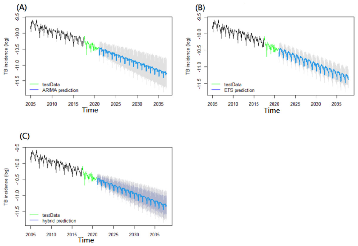
Scheme 1: Long-term predictions for tuberculosis incidence rates until 2030.
(A) SARIMA model, (B) ETS model, (C) SARIMA-ETS hybrid model.
Simulating by an ETS programming function for the time series datasets of 192 monthly tuberculosis incidence rates, an ETS(A,A,A) model was appropriated to be captured (AIC = −46.107399, AICc = −42.306157, BIC = 8.078159; Dickey-Fuller = −9.9554, Lag order = 1, p-value = 0.01, stationary) (Dickey-Fuller = −9.9554, Lag order = 1, PDickey-Full = 0.01, alternative hypothesis: stationary; Ljung-Box test, data: Residuals from ETS(A,A,A), Q* = 56.673, df = 8, PBox-Ljung = 2.086e−09, Model df: 16, Total lags used: 24) (Table 1).
While establishing the ARIMA-ETS-hybrid models, a combined model comprised of weight 0.5 of ARIMA and weight 0.5 of ETS was constructed. The outcomes were subsequently calculated.
Projection of TB incidence
Base on the verification of each best-fitting model, we paralleled utilizing the time series of 192 datasets to a long-distance projecting of forecasting for the future. The future TB incidence rates were predicted, which was projecting ahead to the future forecasting more than 3 years over the next several years. After exponentiating the resulting logarithmic TB incidence values, the projection outcomes of the next several-year TB incidence rates based on the outcome of ETS with best performance than SARIMA-ETS and SARIMA was 26.586 (95% CI [21.601–32.721]) per 100,000-year in 2025 and 20.706 (95% CI [16.328–26.258]) per 100,000-year in 2030 (Table 3, Scheme 1). Moreover, the projection outcome of the future-year TB incidences based on the ETS model showed a 41.82% (range: 28.40–52.72%) reduction in 2025 and a 54.69% (range: 42.54–54.77%) reduction in 2030 compared with 2015 levels (Table 3, Scheme 1).
| ARIMA | ETS | ARIMA-ETS-hybrid | |||||||
|---|---|---|---|---|---|---|---|---|---|
| Year (reduction*) | TB incidence: TB cases per 100,000-year (*) | TB incidence: TB cases per 100,000-year (*) | TB incidence: TB cases per 100,000-year (*) | ||||||
| Forecast value | Lo. 99.5% | Hi. 99.5% | Forecast value | Lo. 99.5% | Hi. 99.5% | Forecast value | Lo. 99.5% | Hi. 99.5% | |
| 2021 | 32.380 | 26.317 | 39.839 | 32.471 | 27.016 | 39.028 | 32.495 | 27.589 | 38.150 |
| 2022 | 31.052 | 24.818 | 38.853 | 30.888 | 25.547 | 37.345 | 30.762 | 25.618 | 36.769 |
| 2023 | 29.261 | 23.008 | 37.214 | 29.382 | 24.158 | 35.735 | 29.331 | 23.790 | 36.121 |
| 2024 | 27.955 | 21.298 | 36.695 | 27.949 | 22.844 | 34.195 | 27.875 | 22.102 | 35.054 |
| 2025 | 26.646 (41.69%) | 19.933 (56.38%) | 35.620 (22.06%) | 26.586 (41.82%) | 21.601 (52.73%) | 32.721 (28.40%) | 26.531 (41.95%) | 20.561 (55.01%) | 34.138 (25.30%) |
| 2030 | 20.803 (54.48%) | 14.286 (68.74%) | 30.294 (33.71%) | 20.706 (54.69%) | 16.328 (64.27%) | 26.258 (42.54%) | 20.671 (54.77%) | 14.636 (67.97%) | 29.138 (36.24%) |
Note:
*Reduction = (Final incidence rate−incidence rate in 2015)/incidence rate in 2015. WHO milestone and targets for TB incidence rate reduction in 2020, 2025, 2030 and 2035 by 20%, 50%, 80% compared with the 2015 (Int J Tuberc Lung Dis. 2018 Jul; 22(7): 723–730.).
Discussion
Our time series analysis for Taiwan TB incidence exhibited a distinct declining trend from 72.5 to 33.2 cases per 105/year, 2005–2020, which was of intermediate burden and considered lower than the global average might be somehow due to the ongoing improvement of efforts and national health policymaking in recent years. The time series was decomposed to examine the seasonal trend and specific patterns. It exhibited that the TB incidence in Taiwan had a steady declining trend having seasonal variation with two peaks occurred mostly in March, April, and May and a trough commonly in November to February. These fluctuations revealed peaks in the early spring might be due to TB dissemination attributed to overcrowding and poor ventilation while the population movement across the cities and people maintained most social activities indoors during the winter Lunar New Year festival in Asia. In addition, the observed TB seasonality of trough periods might be attributed to the length of the TB latent period or monitor manipulating gap which needed to be confirmed by further investigation.
We converted time series data sets as a logarithmic format to smooth the volatility in this study. Subsequently, by the processing of Autocorrelation Function (ACF), Partial Autocorrelation Function (PACF), and a Dickey-Fuller test or a Ljung-Box test with both PDickey-Full and PLjung-box < 0.05 which we determined the TB time series as in a stationary and dependently distributed manner with serial correlation, i.e., rejected H0: the data series was independently distributed (Table 1). In terms of applying the SARIMA, ETS, and SARIMA-ETS-hybrid models to simulate TB epidemics and predict the TB incidence in the future years in Taiwan, several strategies were taken in establishing the models for minimizing the possibility of overfitting or underfitting. For avoiding the overfitting problem as much as possible, we utilized a relatively large sample size of 192 monthly data. Underfitting occurs when a constructed model cannot adequately capture the underlying structure of the data sets. Our modelling exhibited the residuals were confirmed with PLjung-box < 0.05, and good in accuracy metrics of modelling performance implied a low possibility of underfitting in the model. The process of validation was repeated automatically until the optimized model was obtained by R programming (Table 1). Also, for highlighting the performance accuracy of developed ARIMA, ETS, and Hybrid models, we divided the TB time series sample into the first 80% of the data, Jan 2005–Jun 2017, as a training set for in-sample simulated modeling, and the rest 20% of the data, Jul 2017–Dec 2020, as a testing set for pseudo-out-of-sample forecasting tests. Based on these modellings’ accuracy metrics of <1 including the root mean square error (RMSE), mean absolute percentage error (MAPE), mean absolute error (MAE), and mean absolute scaled error (MASE), it revealed that the performance of forecasting models was better than naive random walking both during Jan 2005–Jun 2017 in-sample simulating or during Jul 2017–Dec 2020 pseudo-out-of-sample forecasting. Furthermore, the accuracy metrics of pseudo-out-of-sample forecasting exhibited that all of the forecasting performances of 3–12 months ahead was smaller and better than that of medium term of 18–30 months ahead (Table 2). Also, the accuracy metrics showed the established models were neither overfitting, i.e., good performance on the training data, poor generliazation to other data as well as nor underfitting i.e., poor performance on the training data and poor generalization to other data. Hence, it concluded that our established algorithms exhibited the model’s performance was promising its ability to predict the future in the validation period. And, it showed a more accurate in short-term (<1year ahead) underlying trends of TB incidences than in medium-term (1–3 years ahead) forecasting. Moreover, the SARIMA-ETS-hybrid forecasting model had a superior performance than SARIMA for short-term prediction and could play a role in developing imminent epidemic warnings within a short term of 3–12 months ahead. Overall, the MAPE values among 3–12 months ahead of 0.5% around which was smaller than 0.6% around of 18–30 months ahead and both with similar trends of a gradually widening prediction’s confidence range with time horizon lasting. And ARIMA-ETS hybrid outperformed ARIMA and ETS in short term predictions i.e., under 18 months as well as ETS having the best performance and ARIMA-ETS better than ARIMA among more than 18 months. By comparing the performances of the three models, ARIMA-ETS model having the best metrics with the lowest MAPE in short term prediction of within 18 months ahead periods, otherwise; ETS model with better performance in medium term prediction beyond 18–30 months. To overcome these problems, our and other’s hybrid ETS-ARIMA (exponential smoothing - autoregressive integrated moving average model) (Hyndman, 2006) was promising to improve the forecasting abilities. And, our predictions with gradually widen 95% confidence interval ranges which implied that the short term predictions were always better than medium-term or long-term ones (Table 2).
The global TB epidemic is moving toward a future world of TB-free, i.e., zero deaths and suffering due to the end of TB. To achieve the “End TB” goal, accurate prediction of TB incidence models and algorithms could offer as one of the beneficial tools for effective TB prevention and control practice. According to our analysis, the prevention and control measures to date have been effective in achieving the TB control milestone in 2020; furthermore, it anticipated a reduction in tuberculosis incidence by nearly 50% in 2025 relative to the 2015 level. Indeed, for accelerating to achieve the goal’s TB ending, the attention on strengthening the comprehensive intervention strategies is needed e.g., proactively exploring new effective prophylactic methods for TB; constantly intensifying to improving measurements of vaccination, advanced diagnostics, therapeutics, management of TB comorbidities, and the actualization of universal health coverage and social protection. In our study, it showed that the shorter-term forecast was much more acceptable than the long-term prediction according to the forecast’s range confidence values was gradually widening with the growing time companying with the dynamics of TB interventions or the changing Taiwan demographics in the future. Thus, observational data series should be updated overtime to ensure that the forecasting model provides for the best prediction possibly in the practice. According to our outcomes it showed that the SARIMA, ETS and SARIMA-ETS had proven to be sufficiently accurate in the short term or medium term predictions i.e., under 1 year ahead or 3 years ahead, Jul 2015–Dec 2020. Otherwise, the outcomes in the long term should be deemed with more caution because of the unavoidable uncertainly and bias which might occur over time. Nevertheless, we conclude that our time series modellings for TB incidence rate prediction with performance accuracy metrics were the promising tools for facilitating forecasting future vision.
Limitations
There are some limitations to our forecasting models. First, the predictivity of our models decreased with longer time distances, and the confidence interval become wider, suggesting that our models are better at predicting the near epidemics than the long-term trend prediction. By integrating the forecasts and manipulating process by human judgment for future epidemics might restructure the working states. Second, using other new deep learning algorithms, may help to improve the forecasting accuracy.
Conclusions
In summary, the time series analysis assists us in interpreting the historical trends of tuberculosis incidence and seasonality, as well as predicting these trends for the future, which may be conducive and instrumental for short-term epidemic warnings soon, resource allocation as well as plans to facilitate the WHO’s long-term goal for TB control and to enhance epidemic preparedness. Although the proposed SARIMA-ETS-hybrid models outperformed the SARIMA model, overall showed better short-term future forecasting than long-term future forecasting.