
UV synchrotron radiation linear dichroism spectroscopy of the anti-psoriatic drug anthralin
- Published
- Accepted
- Received
- Academic Editor
- Walter de Azevedo Jr.
- Subject Areas
- Spectroscopy, Theoretical and Computational Chemistry, Photochemistry, Physical Chemistry
- Keywords
- Anthralin, Electronic transitions, Polarization spectroscopy, Linear dichroism (LD), Excited state intramolecular proton transfer (ESIPT), Synchrotron radiation, Time-dependent density functional theory (TD-DFT)
- Copyright
- © 2019 Nguyen et al.
- Licence
- This is an open access article distributed under the terms of the Creative Commons Attribution License, which permits unrestricted use, distribution, reproduction and adaptation in any medium and for any purpose provided that it is properly attributed. For attribution, the original author(s), title, publication source (PeerJ Physical Chemistry) and either DOI or URL of the article must be cited.
- Cite this article
- 2019. UV synchrotron radiation linear dichroism spectroscopy of the anti-psoriatic drug anthralin. PeerJ Physical Chemistry 1:e5 https://doi.org/10.7717/peerj-pchem.5
Abstract
Anthralin (1,8-dihydroxyanthrone, 1,8-dihydroxy-9(10H)-anthracenone), also known as dithranol and cignolin, is one of the most efficient drugs in the treatment of psoriasis and other skin diseases. The precise mode of biochemical action is not fully understood, but the activity of the drug is increased by the influence of UV radiation. In the present investigation, the UV absorption of anthralin is studied by synchrotron radiation linear dichroism (SRLD) spectroscopy on molecular samples partially aligned in stretched polyethylene, covering the near and vacuum UV regions with wavenumbers ranging from 23,000 to 58,000 cm–1(430–170 nm). The observed polarization spectra are well predicted by quantum chemical calculations using time-dependent density functional theory (TD–DFT). About a dozen spectral features are assigned to computed electronic transitions. The calculations support interpretation of the anomalous fluorescence of anthralin as a result of barrier-less excited state intramolecular proton transfer (ESIPT) to the tautomer 8,9-dihydroxy-1(10H)-anthracenone.
Introduction
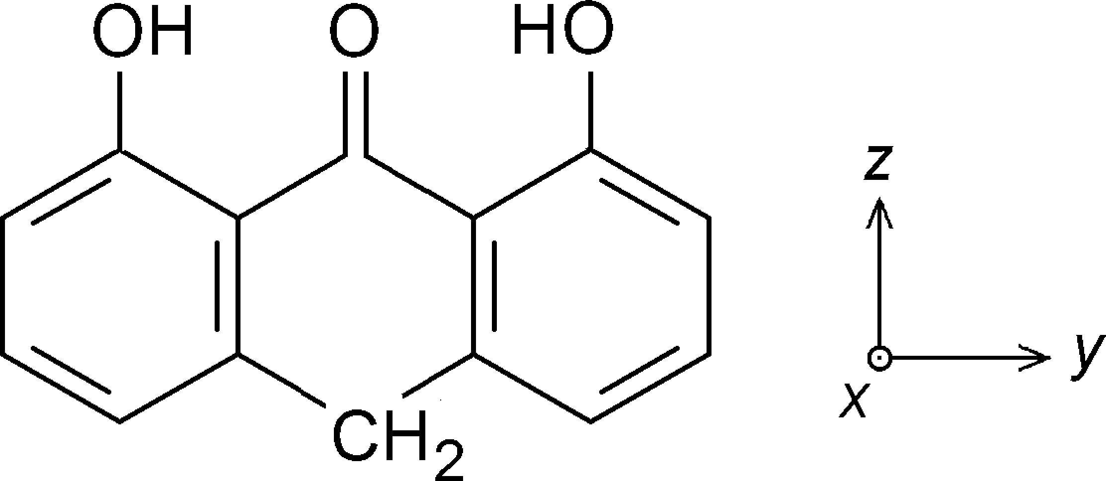
For more than 100 years anthralin (A), also known as dithranol and cignolin, has been applied as an effective topical agent for the treatment of the skin disease psoriasis (Ashton et al., 1983; Van de Kerkhof, 1991; Sehgal, Verma & Khurana, 2014; Körber et al., 2019). The compound was for many years believed to be anthracene-1,8,9-triol, but spectroscopic and crystallographic analyses indicated that the prevailing constitution is that of the tautomer 1,8-dihydroxy-9(10H)-anthracenone (Hellier & Whitefield, 1967; Avdovich & Neville, 1980; Ahmed, 1980), see Fig. 1. A is a reactive compound characterized by complicated red-ox properties (Czerwinska et al., 2006; Pshenichnyuk & Komolov, 2014) and it exhibits anomalous fluorescence with a Stokes shift of 10,500 cm−1, indicating large rearrangement in the excited state (Møller et al., 1998). The precise mode of biochemical action is not fully understood, but the application of UV radiation is known to increase the activity of the drug (Lapolla et al., 2011). Bally and coworkers (Czerwinska et al., 2006) and Pshenichnyuk & Komolov (2014) thus considered the involvement of excited electronic states generated by UV irradiation.
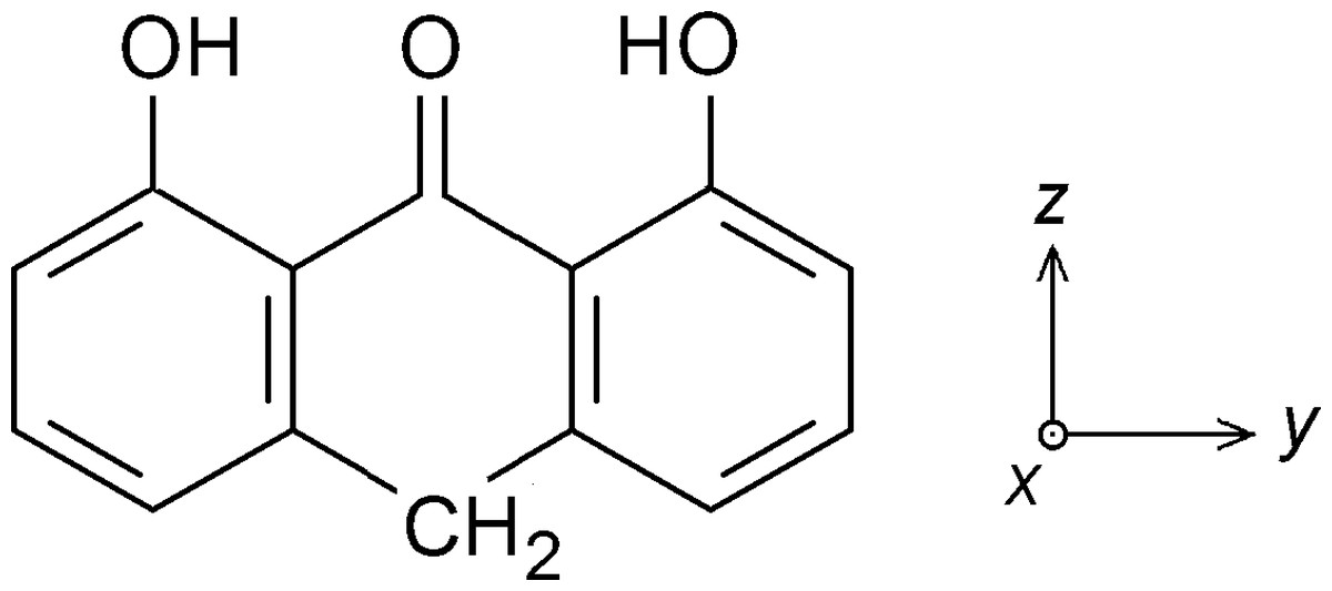
Figure 1: Anthralin (A) with definition of the molecular coordinate system.
In the present work, we investigate the excited states of A by synchrotron radiation linear dichroism (SRLD) UV spectroscopy on molecular samples partially aligned in stretched low-density polyethylene (PE). The use of synchrotron radiation (Miles et al., 2007; Miles et al., 2008) provides increased signal-to-noise ratio in the UV region and enables a significant expansion of the accessible spectral range, compared with the use of a traditional light source (Nguyen et al., 2018; Nguyen et al., 2019). In the present study, the measurement is extended into the vacuum UV, covering the region up to 58,000 cm−1 (170 nm); this is an extension of the previously investigated range by about 11,000 cm−1 (1.4 eV) (Andersen & Spanget-Larsen, 1997). Linear dichroism (LD) spectroscopy yields experimental information on the molecular transition moment directions of the observed absorption bands (Michl & Thulstrup, 1986; Thulstrup & Michl, 1989; Rodger & Nordén, 1997; Nordén, Rodger & Dafforn, 2010). The observed spectra are discussed with reference to the results of time-dependent density functional theory (TD-DFT) calculations (Marques et al., 2012; Foresman & Frisch, 2015). Additional information is provided as Supplemental Files.
Materials & Methods
Sample preparation
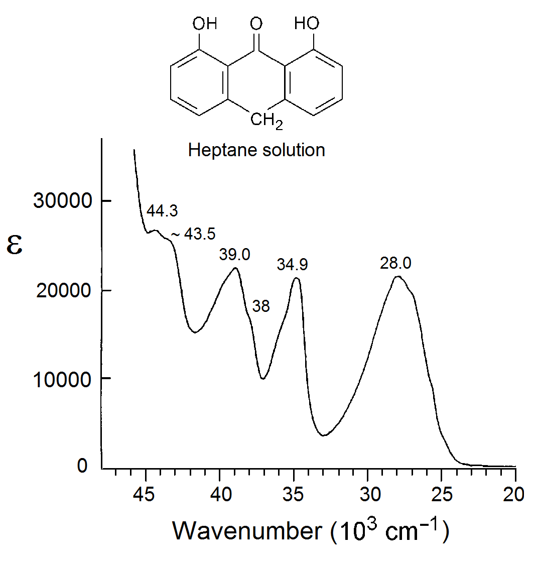
A sample of A (CAS No. 1143-38-0) was purchased from Sigma-Aldrich and purified by column chromatography as previously described (Andersen & Spanget-Larsen, 1997). The near-UV absorbance spectrum of the purified substance in n-heptane solution (Merck Uvasol) is shown in Fig. S1. Low-density polyethylene (PE) 100 µm sheet material was obtained from Hinnum Plast A/S. A 2.5 ×6 cm PE piece cut from the sheet was purified by extraction with chloroform (Merck Uvasol) at 50 °C for one day. A was introduced by submersion of the dried PE sample into a saturated chloroform solution of the substance in a sealed container at room temperature for three days. After evaporation of the chloroform from the doped sample, the surface was cleaned with ethanol (Merck Uvasol) to remove crystalline deposits. The PE sample was finally uniaxially stretched by 500%. A sample without solute was produced in the same manner for use as a reference. Further details on stretched polyethylene samples can be found in the literature (Michl & Thulstrup, 1986; Thulstrup & Michl, 1989).
Linear dichroism (LD) spectroscopy
LD spectra in the range 31,300–20,000 cm−1 (320–500 nm) were recorded on a UV-2101PC Shimadzu spectrophotometer at Roskilde University. SRLD spectra were measured in the range 58,000–31,300 cm−1 (170–320 nm) on the CD1 beamline (Miles et al., 2007; Miles et al., 2008) at the storage ring ASTRID at the Centre for Storage Ring Facilities (ISA). As previously described (Andersen & Spanget-Larsen, 1997; Nguyen et al., 2018; Nguyen et al., 2019), two absorbance curves were recorded at room temperature with the electric vector of the sample beam parallel (U) and perpendicular (V) to the stretching direction of the PE sample. The observed baseline-corrected LD absorbance curves and are shown in Fig. 2A. The isotropic absorbance curve is shown in Fig. S2.

Figure 2: Observed SRLD absorbance curves.
(A) Absorbance curves EU and EV for anthralin (A) partially aligned in uniaxially stretched polyethylene, indicating absorbance measured with linearly polarized radiation with electric vector parallel and perpendicular, respectively, to the stretching direction U of the polymer. (B) Family of reduced absorbance curves rK according to Eq. (2) with K varying from 0.0 to 1.0 in steps of 0.1. Orientation factors K determined for prominent features are indicated. (C) Partial absorbance curves Ay and Az according to Eq. (3) corresponding to absorbance polarized along the molecular axes y and z, see text.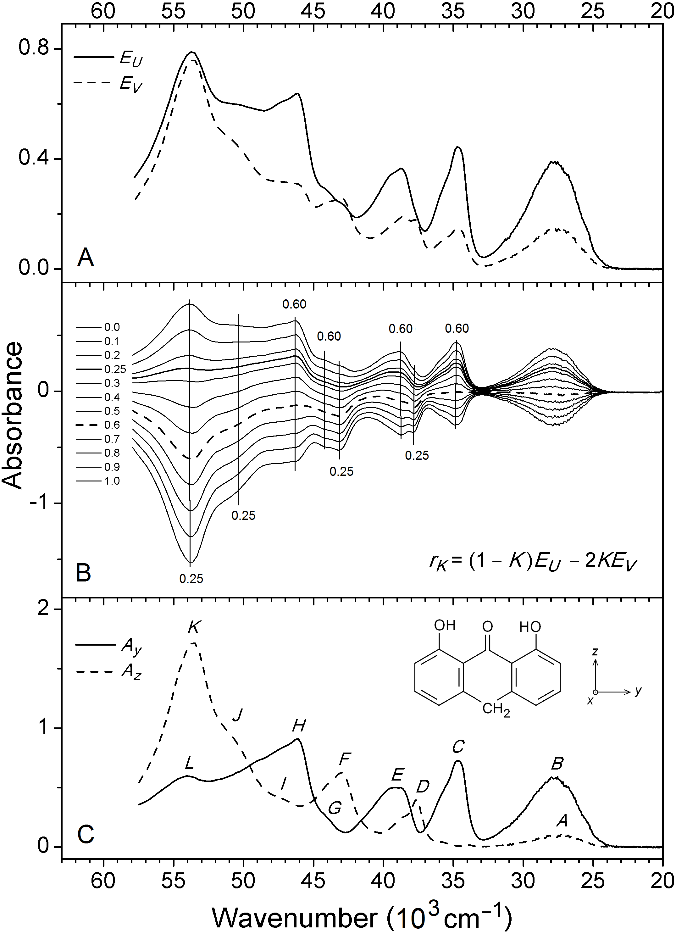
Calculations
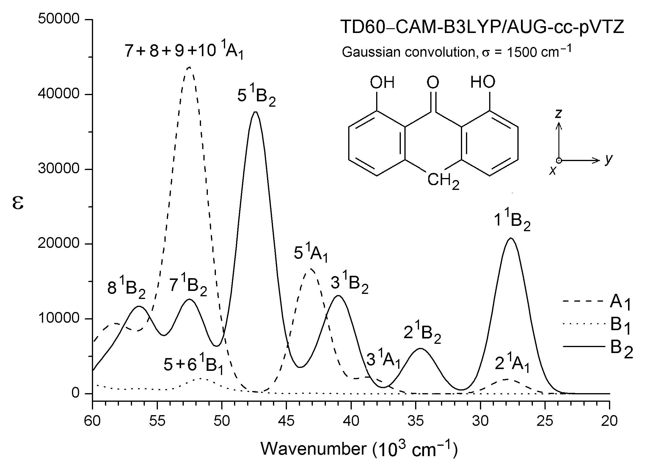
Quantum chemical calculations considering isolated molecules in the gas phase were performed by using the Gaussian16 software package (Frisch et al., 2016). Optimizations of molecular geometry were performed with B3LYP (Becke, 1993; Lee, Yang & Parr, 1988). This DFT was found to be very successful in the prediction of molecular and vibrational structures of compounds like A with intramolecular C=O⋅⋅⋅HO hydrogen bonding (Spanget-Larsen, Hansen & Hansen, 2011; Hansen & Spanget-Larsen, 2012). Geometry optimizations for the ground state (S0) and the lowest excited singlet state (S1) of A were carried out with B3LYP and TD-B3LYP, respectively, using the 6-31+G(d,p) basis set (Foresman & Frisch, 2015; Frisch et al., 2016). Vertical electronic transitions from the ground state to the 60 lowest excited singlet states were computed with TD–CAM-B3LYP (Yanai, Tew & Handy, 2004) and the basis set aug-cc-pVTZ (Dunning Jr, 1989; Kendall, Dunning Jr & Harrison, 1992). We recently found that this long-range corrected procedure is adequate in the prediction of electronic transitions of aromatic chromophores in the near and vacuum UV regions (Nguyen et al., 2018; Nguyen et al., 2019). A constant term was subtracted from the excitation wavenumbers calculated with TD–CAM-B3LYP in order to facilitate comparison with the observed spectra (Grimme, 2004; Nguyen et al., 2018; Nguyen et al., 2019); an empirical correction of 3,500 cm−1 was found to be adequate in the present case. The main predicted transitions are listed in Table 1 together with the observed ones. A complete listing of the calculated transitions is provided as Data S1. Graphical representations of transitions to 1A1 and 1B2 states are shown in Fig. 3. Gaussian convolutions considering all allowed transitions are provided as Fig. S3, using previously described procedures (Serr & O’Boyle, 2009; Nguyen et al., 2019). Detailed results for the ESIPT photoproduct 8,9-dihydroxy-1(10H)-anthracenone are given in Data S2, results for additional excited state configurations are outlined in Fig. S4.
| Observed | TD–CAM-B3LYPa | |||||||
|---|---|---|---|---|---|---|---|---|
| b | Absc | Pol d | Term | b,e | ff | Leading configurationsg | ||
| A | 27.3 | 0.11 | z | 2 1A1 | 27.9 | 0.03 | 93% [6b1(π) →7b1(π*)] | |
| B | 27.7 | 0.58 | y | 1 1B2 | 27.7 | 0.29 | 94% [4a2(π) →7b1(π*)] | |
| C | 34.6 | 0.73 | y | 2 1B2 | 34.6 | 0.08 | 79% [3a2(π) →7b1(π*)], 13% [6b1(π) →5a2(π*)] | |
| D | 37.6 | 0.39 | z | 3 1A1 | 38.6 | 0.03 | 73% [5b1(π) →7b1(π*)], 13% [6b1(π) →8b1(π*)] | |
| E | 39.2 | 0.50 | y | 3 1B2 | 40.9 | 0.18 | 54% [6b1(π) →5a2(π*)], 17% [3a2(π) →7b1(π*)] | |
| F | 42.9 | 0.62 | z | 5 1A1 | 43.2 | 0.23 | 56% [6b1(π) →8b1(π*)], 21% [5b1(π) →7b1(π*)] | |
| G | 44 | (0.2) | y | 4 1B2 | 43.5 | 0.03 | 55% [4a2(π) →8b1(π*)], 23% [6b1(π) →6a2(π*)] | |
| H | 46.1 | 0.91 | y | 5 1B2 | 47.4 | 0.52 | 29% [3a2(π) →8b1(π*)], 19% [6b1(π) →6a2(π*)] | |
| I | 47 | (0.4) | z | 7 1A1 | 50.9 | 0.06 | 43% [6b1(π) →9b1(π*)], 16% [5b1(π) →8b1(π*)] | |
| J | 51 | (1.0) | z | 8 1A1 | 52.1 | 0.17 | 21% [5b1(π) →8b1(π*)], 19% [4b1(π) →7b1(π*)] | |
| K | 53.4 | 1.72 | z | 9 1A1 | 52.8 | 0.41 | 53% [4a2(π) →6a2(π*)], 30% [3a2(π) →5a2(π*)] | |
| 10 1A1 | 55.3 | 0.09 | 66% [4b1(π) →7b1(π*)], 12% [5b1(π) →8b1(π*)] | |||||
| 12 1A1 | 57.9 | 0.08 | 54% [3a2(π) →6a2(π*)], 29% [5b1(π) →8b1(π*)] | |||||
| L | 54.1 | 0.60 | y | 8 1B2 | 52.5 | 0.16 | 34% [3a2(π) →8b1(π*)], 29% [5b1(π) →5a2(π*)] | |
| 9 1B2 | 56.3 | 0.14 | 50% [2a2(π) →7b1(π*)], 12% [22b2(σ) →30a1(σ*)] | |||||
Notes:

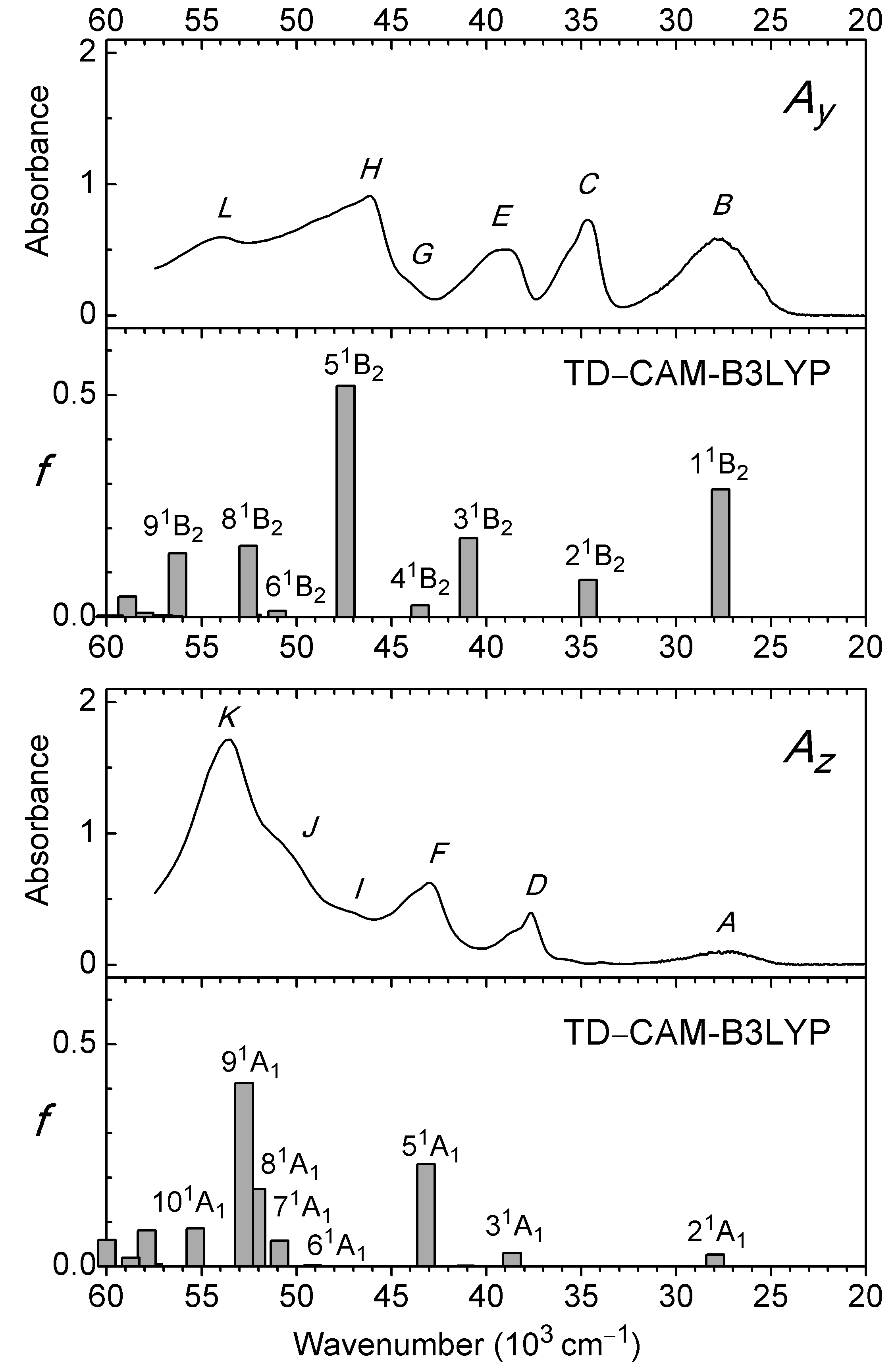
Figure 3: Partial absorbance curves Ay and Az for anthralin (A) and electronic transitions to excited 1B2 and 1A1 states predicted with TD–CAM-B3LYP/aug-cc-pVTZ.
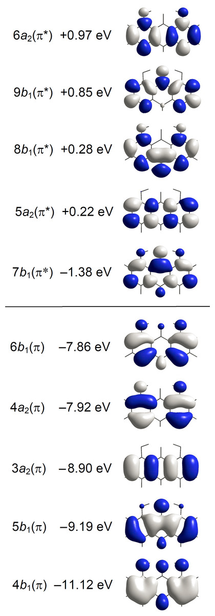
Figure 4: Energies and amplitude diagrams for the five highest occupied and five lowest unoccupied π type MOs of anthralin (A) computed with CAM-B3LYP/aug-cc-pVTZ.
Different colors indicate amplitudes of different sign.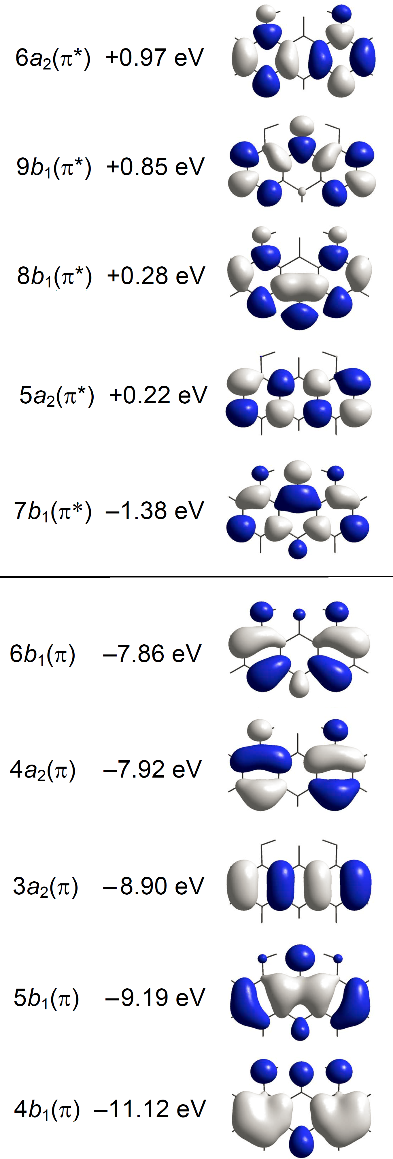
Results and Discussion
Linear dichroism: orientation factors and partial absorbance curves
The observed SRLD absorption curves and for A partially aligned in stretched PE are shown in Fig. 2A. The directional information that can be extracted from these curves is represented by the orientation factors Ki for the molecular transition moment vectors of the observed spectroscopic features i (Michl & Thulstrup, 1986; Thulstrup & Michl, 1989): (1)
The orientation factor is defined as an average over all solute molecules in the light path, indicated by the pointed brackets in Eq. (1), where is the angle of the moment vector of transition i with the polymer stretching direction, U. The Ki values may be determined by the graphical TEM procedure (Michl & Thulstrup, 1986; Thulstrup & Michl, 1989) which involves construction of linear combinations of and . In the present application we consider the reduced absorbance curves (Madsen et al., 1992): (2)
A family of curves for A is shown in Fig. 2B. A spectral peak or shoulder due to transition i disappears from the linear combination for K = Ki and the Ki value can thus be determined by visual inspection. The molecular point group of A is C2v (Ahmed, 1980) and allowed vertical transitions must be polarized along the three symmetry axes x, y, and z, corresponding to excited states of B1, B2, and A1 symmetry, respectively. Hence, only three different Ki values corresponding to Kx, Ky, and Kz are expected. From the curves in Fig. 2B K values close to 0.60 can be estimated for the features at 34,600, 39,200, 44,000 and 46,100 cm−1, and values close to 0.25 for those at 37,600, 42,900, 51,000 and 53,400 cm−1. As previously discussed (Andersen & Spanget-Larsen, 1997), the relatively broad band with maximum close to 27,500 cm−1 (∼365 nm) is due to two near-degenerate, differently polarized transitions; their K values cannot be determined directly.
The K values 0.60 and 0.25 must be assigned to Ky and Kz, corresponding to transitions polarized along the in-plane long and short molecular axes y and z. Under the assumption that absorbance polarized along the out-of-plane x axis is negligible in the present spectra, it is possible to construct the partial absorbance curves and indicating y- and z- polarized intensity (Madsen et al., 1992):
(3)
The curves and produced with (Ky, Kz) = (0.60, 0.25) are shown in Fig. 2C and in Fig. 3. They are shown on an expanded absorbance scale in Fig. S2, together with the isotropic absorbance curve . The latter is equal to three times the absorbance that would have been measured in an isotropic experiment on the same sample. Six long-axis (y) polarized features B, C, E, G, H, and L and six short-axis (z) polarized features A, D, F, I, J, and K are indicated. Observed peak wavenumbers, absorbances, and polarization directions are listed in Table 1.
Electronic transitions
The spectrum starts with a relatively broad band system with maximum close to 27,500 cm−1 (364 nm). The absorbance is predominantly long-axis (y) polarized, overlapping weaker short-axis (z) polarized intensity. The short-axis polarized absorbance A with maximum at 27,300 cm−1 (366 nm) can be assigned to the 21A1 state computed at 27,900 cm−1 (Table 1, Fig. 3). The computed transition is well described by promotion of an electron from the 6b 1(π) HOMO to the 7b 1(π*) LUMO. The intense long-axis polarized band B peaking at 27,700 cm−1 (361 nm) is assigned to the 11B2 state predicted at 27,700 cm−1 (Table 1, Fig. 3). This transition is primarily due to the promotion from the 4a 2 (π) SHOMO to the 7b 1(π*) LUMO.
Band C with maximum at 34,600 cm−1 (289 nm) is purely long-axis (y) polarized and is easily assigned to the 21B2 state computed at 34,600 cm−1 (Table 1, Fig. 3). The following absorbance band is resolved into two differently polarized components, D and E at 37,600 and 39,200 cm−1 (266 and 255 nm). They can be assigned to the 31A1 and 31B2 states computed at 38,600 and 40,900 cm−1 (Table 1, Fig. 3). Band F at 42,900 cm−1 (233 nm) is predominantly short-axis (z) polarized and is assigned to the 51A1 state predicted at 43,200 cm−1 (Table 1, Fig. 3). The band overlaps the onset of long-axis polarized (y) intensity G around 44,000 cm−1 (∼227 nm). This feature is possibly due to the 41B2 state computed at 43,500 cm−1 (Table 1, Fig. 3), but it may also involve b 2 symmetric vibrational components of band F, gaining long-axis polarized intensity by vibronic coupling with the strong band H. In the isotropic spectrum recorded in n-heptane solution, transition F apparently corresponds to the shoulder close to 43,500 cm−1 and transition G to the peak at 44,300 cm−1 (Fig. S1).
Assignment of individual transitions in the high-wavenumber region is complicated by the presence of broad, overlapping bands and by a high density of electronic states. Our TD–CAM-B3LYP calculation predicts about 50 electronic transitions between 60,000 and 45,000 cm−1 (Data S1). In addition, the applied theoretical model may be less accurate in this region and the suggested assignments of observed features to computed transitions are necessarily tentative.
The observed long-axis (y) polarized absorbance in this region displays a strong band H with maximum at 46,100 cm−1 (217 nm). According to the calculated transitions, this band can be assigned to the 51B2 state predicted at 47,400 cm−1 (Table 1, Fig. 3). Band H has a long tail into the vacuum UV with an additional peak L at 54,100 cm−1 (185 nm). Several states are predicted to contribute to this absorption, primarily 81B2 and 91B2 computed at 52,500 and 56,300 cm−1 (Table 1, Fig. 3).
The short-axis (z) polarized intensity in this region is dominated by a very strong band K with maximum at 53,400 cm−1 (187 nm) in the vacuum UV. This is the strongest absorbance observed in the investigated spectral range. The peak K at 53,400 cm−1 is preceded by two diffuse shoulders I and J at 47,000 and 51,000 cm−1 (213 and 196 nm). Several states are predicted to contribute to this band system, such as 71A1, 81A1, 91A1, and 101A1, with transition to the 91A1 state computed at 52,800 cm−1 as the most intense (Table 1, Fig. 3).
Excited state intramolecular proton transfer (ESIPT)
The observed fluorescence emission of A in n-hexane solution has a maximum at 17,500 cm−1 (570 nm) with an unusually large Stokes shift of 10,500 cm−1 relative to the excitation observed at 28,000 cm−1 (360 nm) (Møller et al., 1998). The fluorescence quantum yield is nearly independent of temperature which suggests that the decay from the initially formed excited state to the ground state does not involve barrier crossing (Møller et al., 1998).
According to the orbital amplitudes in Fig. 4, the promotions 6b 1(π) → 7b 1 (π*) and 4a 2(π) → 7b 1(π*) involved in the transitions to the two lowest, near-degenerate singlet states 21A1 and 11B2 are associated with substantial transfer of electron density from the phenolic moieties to the carbonyl group. This is expected to affect the balance of forces involved in the intramolecular hydrogen bonding, facilitating excited state intramolecular proton transfer (ESIPT) (Andersen & Spanget-Larsen, 1997). Geometry optimization of the excited S1 state with TD-B3LYP predicts barrier-less transition to the ESIPT product 8,9-dihydroxy-1(10H)-anthracenone, see Fig. 5, leading to good agreement with the observed fluorescence and excitation wavenumbers (the predicted excitation wavenumber indicated in Fig. 5 is slightly different from the one listed in Table 1 because of different TD-DFT procedures). The present TD-DFT results thus support the assignment previously suggested on the basis of semi-empirical model calculations (Andersen & Spanget-Larsen, 1997; Møller et al., 1998). Excited state equilibrium nuclear coordinates and other computational data for the ESIPT product are provided as Data S2; relative energies of this and additional excited state configurations are outlined in Fig. S4.

Figure 5: Predicted vertical excitation and emission wavenumbers for anthralin (A).
On the left the predicted vertical transition from the ground state to the lowest excited singlet state is indicated, to the right the vertical emission from the photoproduct 8,9-dihydroxy-1(10H)-anthracenone (TD-B3LYP/6-31+G(d,p)). The predicted photoproduct is a result of barrier-less excited state intramolecular proton transfer (ESIPT). Further details are provided in Data S2 and Fig. S4.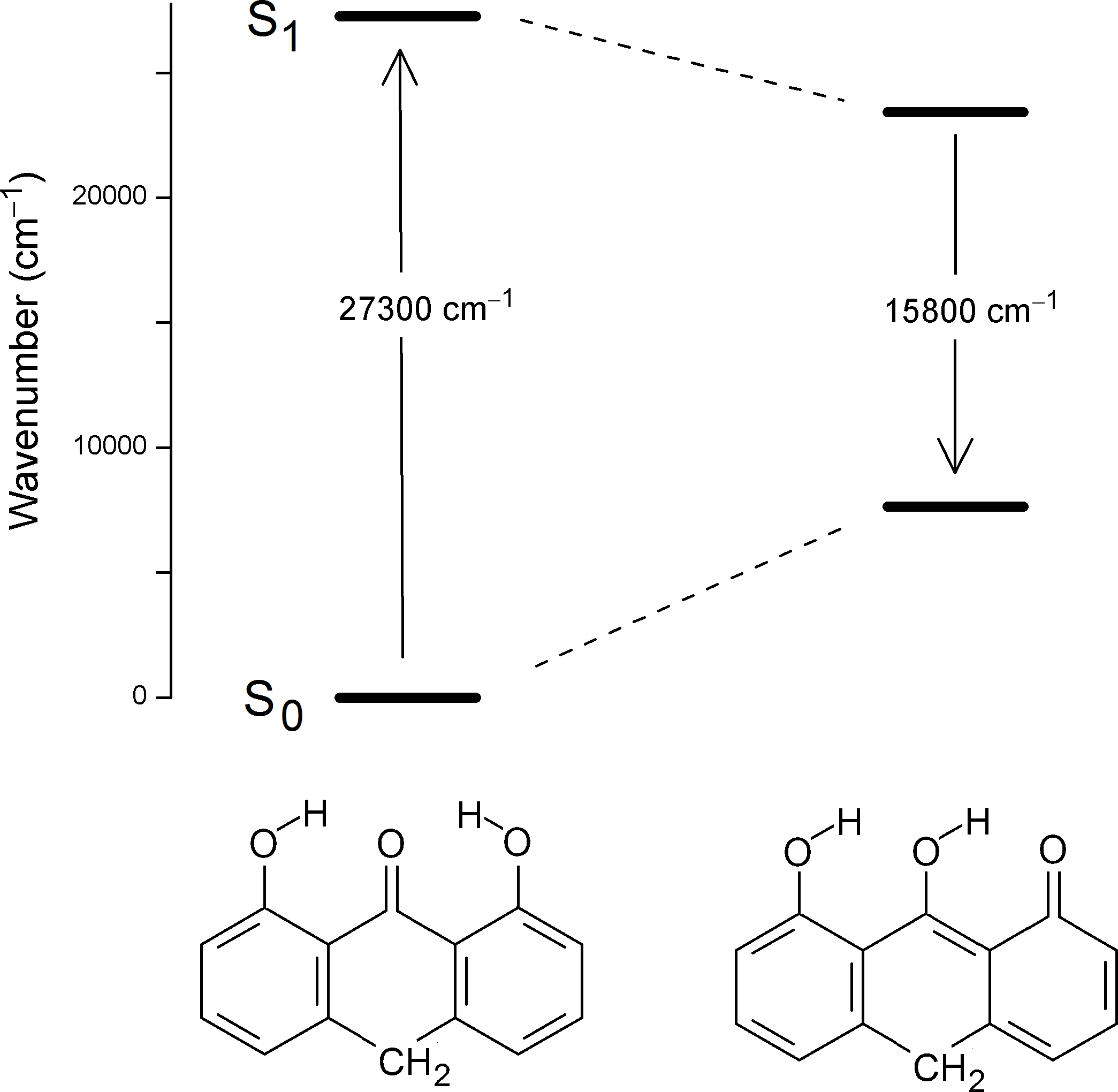
A similar excited state rearrangement is observed for the closely related compound 1,8-dihydroxy-9,10-anthraquinone (chrysazin, an oxidation product of A) as reported by Smulevich and coworkers (Smulevich et al., 1987; Marzocchi et al., 1998) and recently studied theoretically by Mohammed et al. (2014) and by Zheng, Zhang & Zhao (2017).
Conclusions
In this study, polarization data for the anti-psoriatic drug anthralin (A) is provided by SRLD spectroscopy in the region 58,000–23,000 cm−1 (170–430 nm), leading to the resolution of otherwise overlapping absorption bands and to experimental symmetry assignments of the observed transitions. The results of the present TD–DFT calculations account admiringly well for the observed polarization spectra throughout the investigated spectral range, allowing detailed assignments of about a dozen observed spectral features to computed electronic states. Assignment of the anomalous fluorescence of A to the ESIPT product 8,9-dihydroxy-1(10H)-anthracenone is supported by the present theoretical results.
Supplemental Information
Equilibrium geometry of the excited state intramolecular proton transfer (ESIPT) photoproduct 8,9‑dihydroxy-1(10H)-anthracenone computed with TD-B3LYP
SRLD partial absorbance curves Ay and Az and corresponding isotropic curve AISO = Ay + Az = EU + 2EV.
Gaussian convolution of transitions computed with TD-CAM-B3LYP.
Gaussian convolutions according to A. Serr, N. O’Boyle, “Convoluting UV-Vis spectra using oscillator strengths” (July 13, 2009), http://gausssum.sourceforge.net/GaussSum_UVVis_Convolution.pdf.
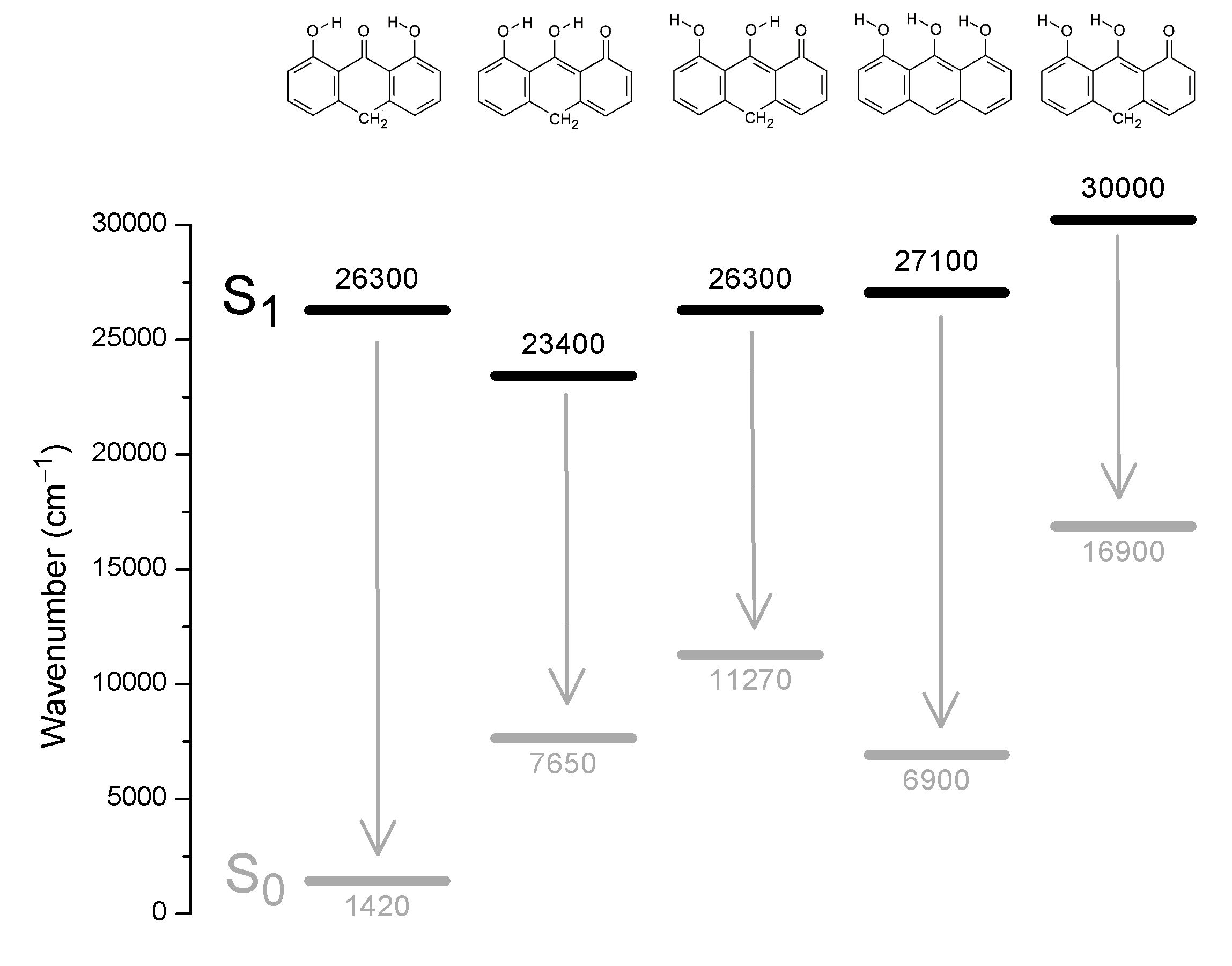
Excited state energies computed with TD-B3LYP/6-31+G(d,p).
The black bars indicate S1 electronic energies in wavenumbers (cm−1) relative to the S0 ground state C2v equilibrium geometry. The arrows indicate vertical transitions corresponding to emission to the S0 ground state. - The excited state geometry of the leftmost configuration was optimized under the restriction of C2v symmetry; this is not an equilibrium geometry, barrier-less transition is predicted to the second leftmost configuration 8,9‑dihydroxy-1(10H)-anthracenone (see also Data S2). The remaining excited state configurations were optimized under the assumption of Cs symmetry.