
Are you ashamed? Can a gaze tracker tell?
- Published
- Accepted
- Received
- Academic Editor
- Pinar Duygulu
- Subject Areas
- Human-Computer Interaction, Artificial Intelligence, Computer Vision
- Keywords
- Cognitive, Recognition, Emotions, Gaze-tracking
- Copyright
- © 2016 Maskeliunas and Raudonis
- Licence
- This is an open access article distributed under the terms of the Creative Commons Attribution License, which permits unrestricted use, distribution, reproduction and adaptation in any medium and for any purpose provided that it is properly attributed. For attribution, the original author(s), title, publication source (PeerJ Computer Science) and either DOI or URL of the article must be cited.
- Cite this article
- 2016. Are you ashamed? Can a gaze tracker tell? PeerJ Computer Science 2:e75 https://doi.org/10.7717/peerj-cs.75
Abstract
Our aim was to determine the possibility of detecting cognitive emotion information (neutral, disgust, shameful, “sensory pleasure”) by using a remote eye tracker within an approximate range of 1 meter. Our implementation was based on a self-learning ANN used for profile building, emotion status identification and recognition. Participants of the experiment were provoked with audiovisual stimuli (videos with sounds) to measure the emotional feedback. The proposed system was able to classify each felt emotion with an average of 90% accuracy (2 second measuring interval).
Introduction
The user interfaces of the future cannot be imagined without an emotion-sensitive modality. More ways other than plain speech are used for communication. Spatial, temporal, visual and vocal cues are often forgotten in computer interfaces. Each cue relates to one or more forms of nonverbal communication that can be divided into chronemics, haptics, kinesics, oculesics, olfactics, paralanguage and proxemics (Tubbs, 2009), relating to certain activities of a human body, voice or gazing. Unfortunately, modern computer-based user interfaces do not take full advantage of nonverbal communicative abilities, often resulting in a much less than natural interaction. Studying classic theories such as (Hess, 1975; Beatty & Lucero-Wagoner, 2000) opens up the idea of eye-tracking for investigating the behavior of the individuals and resulting into the perception of how eye analysis can be used to grasp human behavior from the relationship between pupil responses, various social attitudes and how it might be useful for various other purposes, not excluding diagnostics and therapeutics.
Referring to oculesics as a form of nonverbal communication, we can set a goal of detecting transmissions and reception of significant signals between communicators without the use of pronounced words. Researchers working in the field strongly believe that a Human—Computer interaction might be significantly improved by incorporating social and emotional processes (Kappas & Krämer, 2011). It is clear that vital emotional information might affect human behavior in the context of information technology. However, this area is still somewhat new—progress is starting to become noticeable, ranging from enhancing the naturalness of interfaces to treatments (Bal et al., 2010). Naturally, the emotional part will closely correlate to the eye-based HCIs. Emotional information might be used to attract a user’s attention and then create a favorable atmosphere for subsequent interactions and to increase a user’s willingness to engage in an interaction (Bee, André & Tober, 2009). A recording of visual fixation in nearly real-time can enable us to tell whether individuals express visual attention, are bored or disengaged (D’Mello et al., 2012) or are they tired or fatigued (Nguyen, Isaacowitz & Rubin, 2009).
The manuscript presents an extension of our work on the development of gaze tracking-based emotion recognition system (Viola & Jones, 2004; Raudonis et al., 2013). In other works we have taken a wearable eye tracking device as the main component of an emotion recognition system. Along with a practical task of tele-marketing we are now investigating if it was possible to recognize emotions using a system based on the remote gaze tracking device. Two additional emotional stimuli such as “sensory pleasure” and “shame” were introduced in the analysis framework. “Disgust” and “neutral” emotions were also measured for comparison purposes. The paper presents background analysis, implementation, and concludes with an experimental evaluation.
Background Analysis
Emotions can be categorized into 15 basic emotion stages, which are amusement, anger, contempt, contentment, disgust, embarrassment, excitement, fear, guilt, pride in achievement, relief, sadness/distress, satisfaction, sensory pleasure, and shame. Each of these fifteen stem out to similar and related sub-emotions (Ekman, 1999). The combination of emotions results in a human feeling (Plutchik, 1999). Investigations have shown that eye contact in human-to-human communications play a significant role, where different types of eye motions can represent different emotions. Even non-communicative persons display emotions (Al-Omar, 2013). Anger is associated with glaring and wide open eyes, boredom involves not focusing or focusing to something else, sadness comes with looking down, etc. (Roche & Roche, 2007). This information can be transferred into gaze models based on emotional expressions (Lance & Marsella, 2008). Gaze is influenced by contextual factors such as the emotional expression, as well as the participant’s goal (Kuhn & Tipples, 2011). Cultural differences are affected by contextual information, though the benefit of contextual information depends upon the perceptual dissimilarity of the contextual emotions to the target emotion and the gaze pattern (Stanley et al., 2013).
Novel technological improvements enable the development of affordable, video oculography-based, eye-tracking devices, which were previously available only to a laboratory researcher. These can be divided into two major groups depending on the kind of light used either infrared or visible (Lu, Lu & Yang, 2012). The authors of Christianson et al. (1991) have focused on change dynamics of the pupil (a pupillary response). The study showed that the size of the pupil can change voluntarily or involuntarily. The change in size can result from the appearance of real or perceived objects of focus, and even at the real or guessed indication of such appearances (Calandra et al., 2015). This offers the feasibility of including pupil dilation as a measure to reflect affective states of individuals in the overall emotional intelligence screening system (Al-Omar, Al-Wabil & Fawzi, 2013). The results of Duque, Sanchez & Vazquez (2014) look at gaze-fixation and pupil dilation support the idea that sustained processing of negative information is associated with a higher ruminative style and indicate differential associations between these factors at different levels of depressive symptomatology.
The assessment of attentional orienting and engagement into emotional visual scenes showed that visual attention is captured by displaying both unpleasant and pleasant emotional content (Nummenmaa, Hyönä & Calvo, 2016). Urry (2010), in a randomized within-subjects design, used a cognitive reappraisal to increase and to decrease emotion levels in response to unpleasant pictures and registering gaze focus and direction. The experiments by Budimir & Palmovic (2011) suggested putting emotional content into the figure area and using different non complementary pictures to see if there is a difference between different emotional categories. Lanatà, Valenza & Scilingo (2013) and Calvo & Lang (2004) reported a promising result aimed at investigation of the gaze pattern and variation of pupil size to discriminate emotional states, induced by looking at pictures with different arousal content. Experimental evaluation showed good performance, with better score on arousal than valence (Ringeval et al., 2013). In Soleymani et al. (2012), a combination of EEG and gaze tracking over a display of database of emotional videos (Soleymani, Pantic & Pun, 2012) resulted in the best classification result of 68.5% for three labels of valence and 76.4% for three labels of arousal. These results were obtained using a modality fusion strategy and a support vector machine, demonstrating that user-independent emotion recognition algorithm can outperform individual self-reports for arousal assessments and do not underperform for valence assessments. The authors of Murphya & Isaacowitza (2010) investigated a factor of age, suggesting that age-related gaze patterns in emotion recognition may depend on the specific emotion being recognized and may not be general across stimuli sets.
Implementation
Gaze tracking-based emotion detection method must evaluate an individual motion of the human eye and all changes in its properties carefully representing a certain pathway to a current emotion. Eye motions can be grouped basically into two groups: voluntary and involuntary motions. The eye motion consists of changes in a gaze direction, a change of focus, tracking of an object of interest, etc. These kinds of mostly voluntary controlled motions do not necessarily relate to a current emotional state, but can represent a certain physical status (eg., tired/myopic). In our previous implementations, we have used a head-mounted eye tracking device which captured only a user’s eye. The tracker’s camera was fixed next to a user’s eye and as close as possible thus partly blocking a field of view. This was not a desirable feature, as it created a certain discomfort. We have also noticed that certain participants of our experiments likely did not reveal their true emotion since they found the gaze tracking device unpleasant. The remote eye tracking system does not have such shortcomings and enables capturing “real” (likely) emotions. The authors of the manuscript have decided to investigate two additional emotions which were not investigated in previous works (“shame” and “sensory pleasure”). The section below depicts our ANN based emotion recognition model along with gaze recognition methods, calibration procedure and system workflow. 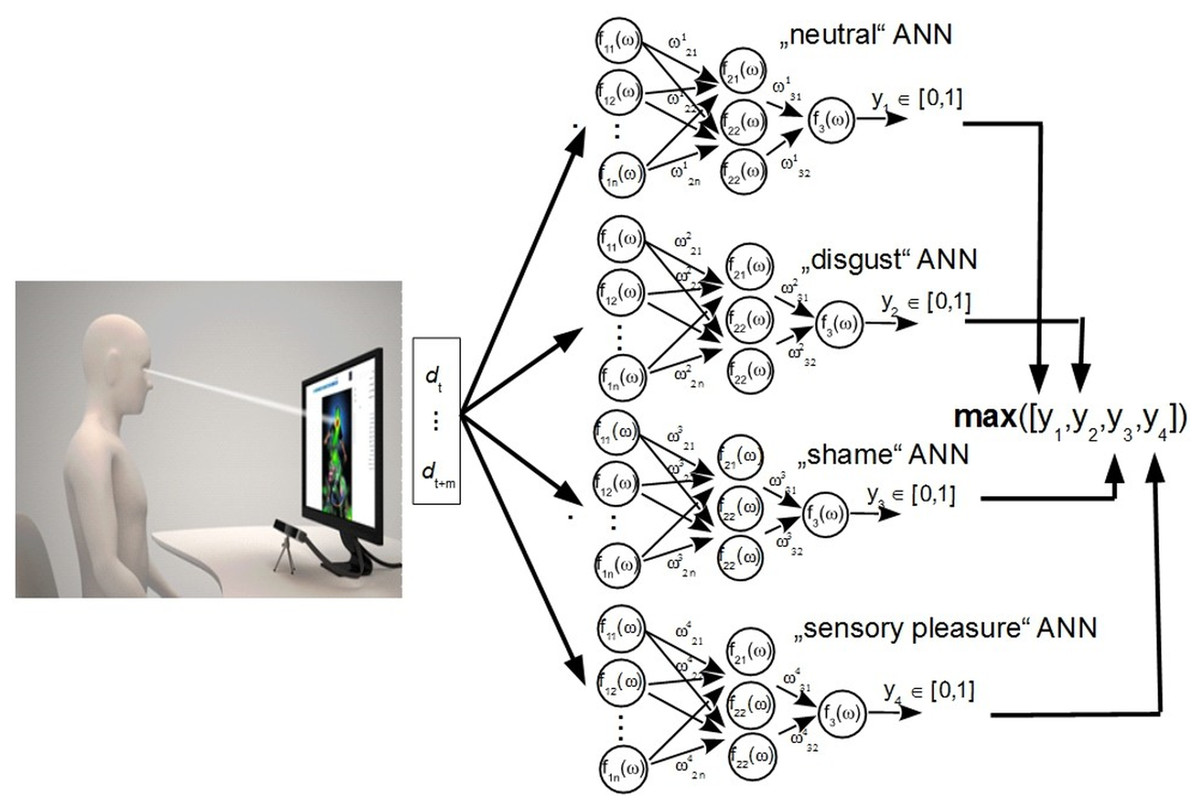
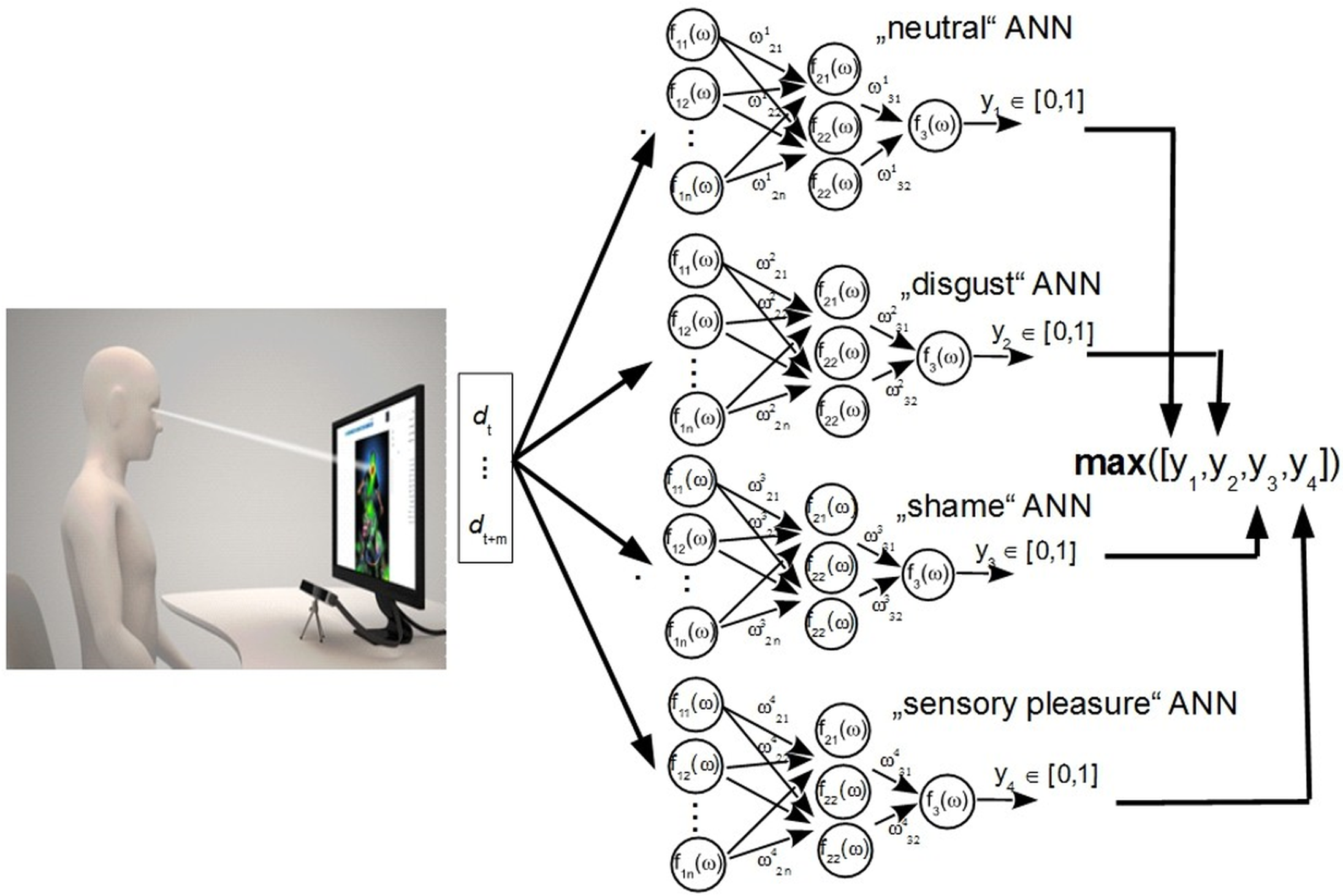
Figure 1: The ANN model and hardware implementation of experimental investigation.
Emotion recognition model
Figure 1 illustrates work flow of an ANN-based classification algorithm. It consists of a measurement device that forms an input vector for four independent neural networks. Each neural network is trained for each individual person to recognize a specific emotional status, i.e., neutral, disgust, shameful or “sensory pleasure.”
The algorithm executes three main steps it: collects data samples, trains a classifier, and makes a decision based on the response of the classifier. The algorithm uses four different neural networks which independently classify given input signals. Levenberg–Marquardt backpropagation was applied as the learning method, activation function served as sigmoid, there were three layers (input layer, hidden layer and output layer). There are 80 neurons onto the first input layer, three neurons on the second hidden layer and one neuron for output. Three features were considered for the ANN networks: the size of the eye pupil d, the position of the gaze point (coordinates x, y) and the motion speed of the gazing point v. The gaze point is the intersection point of gaze vector and the “surface” of the computer screen. Each feature was sampled from 1 to 20 samples per second; therefore, the number of ANN inputs varied. A sample is one measurement taken from one video frame (F). If there is a need for 20 samples, 20 video frames will be measured. One sample includes four parameters: a diameter of the eye pupil (d), a location coordinates of the eye pupil (x, y) and a motion speed on the eye pupil (v), which are taken as a difference between F(t − 1) − F(t). Values of d, x, y and v are used as inputs for neural network. Such combination of values corresponds to one measurement taken from one frame. If we use two measurements (two frames) then a number of inputs will be equal to 4 but not 8 (d1, x1, y1, v_1, d2, x2, y2, d2). An optimal number of inputs was 80 as it corresponded to one second measurement.
Pseudo code of an emotion classification algorithm is presented below.
1. Collecting sample data:
X = ([dt…dt+m][xt…xt+m][yt…yt+m][vt…vt+m−1])
2. Train ANN classifiers based on input data
, wherej = 1, 2, 3, 4
3. Make real-time emotion classification
[maxValue ID] =max(y1, y2, y3, y4);
If maxValue>Threshold
Emotion=ID;
end
Here t—is the time moment at which a sample was recorded, X—the input vector of the ANN, y—output or membership probability, ω–weights of a neural network, d—the diameter of the recognized pupil, xt and yt are the coordinates of the pupil center and vt is the speed of motion of the eye pupils. The final decision is based on a maximal value of membership probability. The recognized emotional state is equal to a network ID that had the highest probability value. We have used a threshold value of 0,5.
Measurements of eye pupil’s center were used for probable capturing of attention focus to a certain extent, as this parameter strongly correlated to the given visual stimuli. ANN finds probable relations to a certain emotion from a coordinate sequence (i.e., several measurements of the pupil’s center).
Gaze tracking methods
The detection and tracking of the human eye was executed in the images acquired in the IR light. The eye illuminated with IR light can give two outcomes: the image of a dark or a bright eye pupil (pupil image and corneal reflection image). The image of a bright pupil is taken when the optical axis of a camera is parallel to the flow of IR light. The image of a dark pupil is taken when optical axis is not parallel to the flow of IR light. Such images are captured in the near IR, which always shows a dark pupil area resulting from the absorption of IR in the inner eye tissues.
The dark pupil effect is used in our eye pupil tracking system. Such an effect simplifies eye pupil detection and the tracking task to a more reliable detection of the dark and rounded region in the image. An initial size of the eye pupil in the image is not known at the starting moment, because the eye pupil has relatively high size variation range. The size variation limits are well known (Iskander et al., 2004) and this a priori information is incorporated in the eye pupil detection algorithm. Presented algorithm uses a notation Rmin and Rmax for describing the lower and upper limits of the eye pupil (or radius).
In this paper we have used a commercial remote eye tracking system hardware (Eye Tribe, Copenhagen, Denmark; https://theeyetribe.com/products/) which is based on one camera sensor and two IR light sources. Acquired images were processed using our own software. The process was based on three fundamental steps:
-
detection of an accurate pupil position;
-
detection of a corneal reflection;
-
finding the relationship between a gaze point and a displacement of the eye pupil position.
The accurate eye pupil and Purkinje reflection is detected by evaluating statistical values of the grey scaled image, i.e., average values of greyness μ and standard deviation σ grey color in the region of interest. These statistical values are computed on the basis of formulas (2) and (3). The accurate detection of an intersection point between the surface of the screen and the gaze vector strongly relies on the calibration procedure and conditions. The calibration ensures a relation between the gaze point (X, Y coordinates on a computer screen) and a pupil position in a captured frame. The grey scaled image is computations are based on formula (1). The pixel value of the grey scaled image is acquired by computing an average color of the three color channels. (1) Here is a color image of the three color channels k = 1, 2, 3. The notations u and v describe coordinates of the image pixel in the matrix.
The average greyness value of region of interest (ROI) can be computed via (2). (2)
The standard deviation of the greyness of ROI is computed using formula (3). (3) Here U and V relate to a total number of rows and columns in the image. Calculated statistical parameters are further used for position detection of the eye pupil and a corneal reflection.
The dark pupil region is detected by estimating a mean greyness value and the standard deviation of each new eye image taken by a remote gaze tracker. Each pixel of an eye image is labeled on the basis of estimated statistics of a functional condition given in formulas (6) and (7). The resulting image Mp that maps the location of a dark region of the eye pupil is estimated regarding condition (6). The black and white image Mr that maps the location of reflection point is estimated using a condition (7). (4) (5)
Examples of the resulting mapping (eye pupil and three reflection points) are shown in Fig. 2.

Figure 2: Grayscaled image G(u, v), and resulting mapping of the Mp and Mr.
The eye pupil is detected in a mapping image Mp. Each resulting point cloud in Mp is measured. The geometrical properties such as geometrical center and area of the cloud (region) are evaluated. The resulting regions in Mp often form simple polygons made of flat shapes consisting of straight, non-intersecting line segments which are joined pairwise to form a closed path. Therefore, formula (6) can be applied to estimate the area of such region. (6)
Here x(i) and y(i) are vertices of a simple polygon. The coordinates of the geometrical center C (described as C = (Cx, Cy)) of the polygons, can be defined as: (7) (8)
Here a total number of polygons j is defined as 0 < j < J − 1.
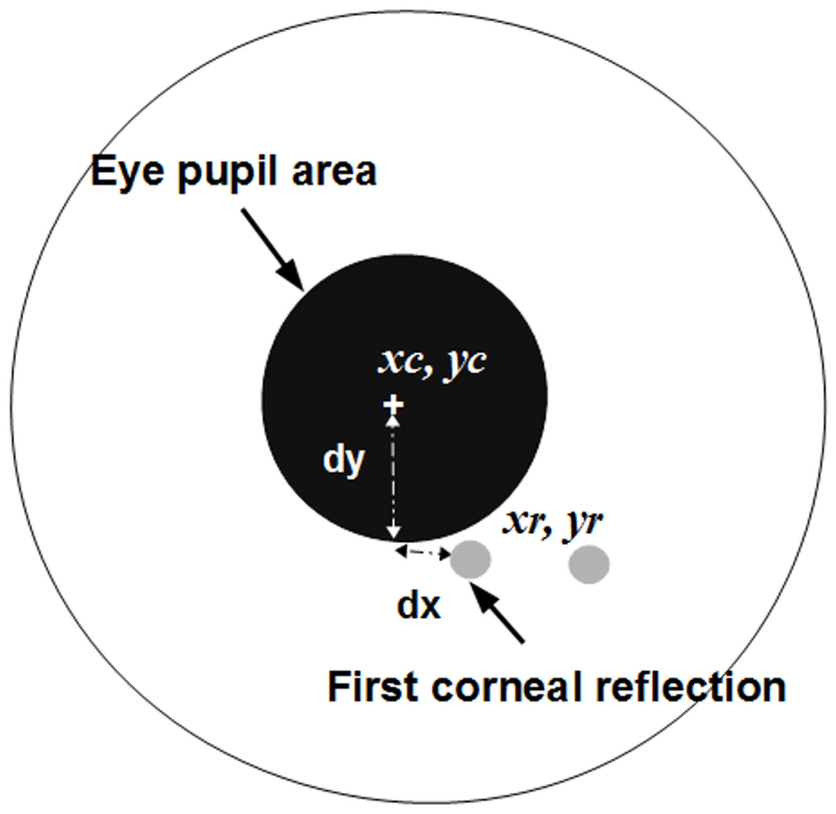
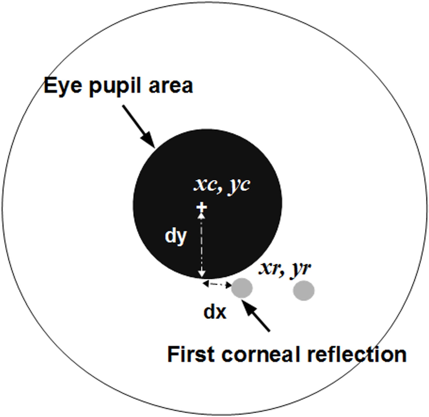
Figure 3: The eye iris and measurements to calculate a gaze point.
In (7), (8) and (9) vertices are numbered in a sequence, from the vertex x(0), y(0) to x(N), y(N). The jth region is labeled as the region that belongs to the eye pupil if it satisfies the condition (9). (9) Here is a minimal limit of the eye pupil size and is a maximum limit of the pupil size. Notations xc and yc denote center coordinates of the detected eye pupil. When the pupil’s center is detected, the first closest reflection point is searched for in the mapping image Mr. There are k points in Mr, and the distance to each point can be expressed as: (10)
Coordinates of the corneal reflection xr and yr are estimated by finding a minimal distance Dr using an expression (13). (11)
The resulting gaze point is obtained by interpolating locations of the pupil’s center and the first corneal reflection. The Fig. 3 illustrates measurements aimed to interpolate the actual intersection point between the gaze vector and the surface of the screen. Displacement values are used for the calibration process. The displacements along horizontal axis and vertical axis can be calculated as: (12)
The linear approximation to a gaze point can be expressed as: (13)
Here X and Y are coordinates of a cursor on a computer screen. Using the method of the least squares a coeficient is calculated by minimazing an error function E(a). (14)
The speed is defined as a simple sum of differences (15). Positive and negative values show the direction in which the gaze is moving. Therefore, a negative value of speed represents only a direction of gazing and how rapidly it changes. (15)
The algorithm has an additional feature to capture out-of-bounds event, in which the extreme turn of the user’s head must be detected to signal the main recognition system to opt-out an event where a user has turned his head away from the computer screen (to capture a “look over the shoulder” effect). Such head motions were often noticeable when participants were stimulated by “shame” and “disgust” emotional stimuli. We have implemented this using standard HAAR cascades to detect a face (Viola & Jones, 2004). When two eyes were visible, a system counted that a user was in the range of tracking fields, otherwise an out of bound event was generated.
Calibration
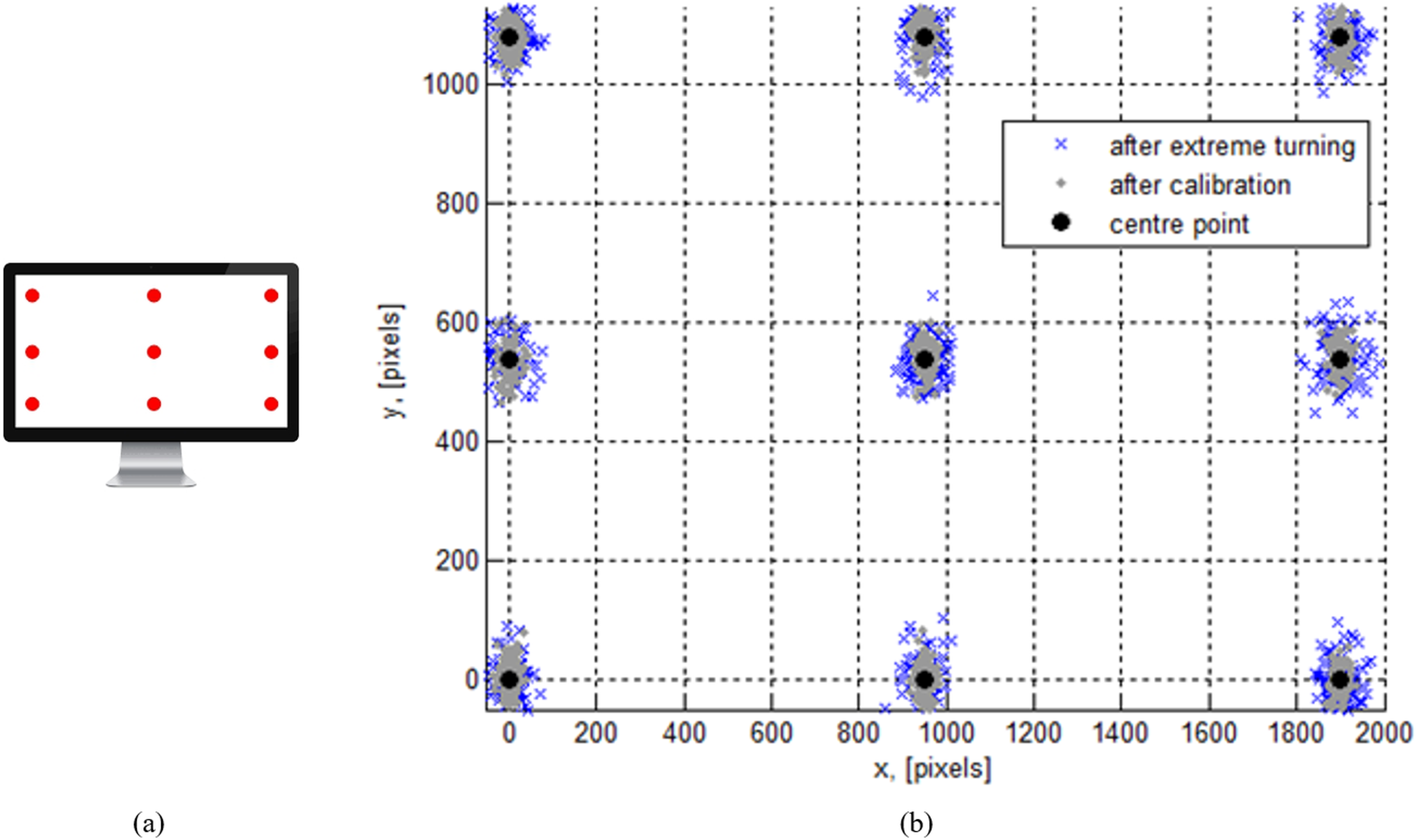
The calibration method is a set of processes that establish a relationship between the center gaze point and an actual position of the computer screen. For the experiment, a 24” 1080p monitor has been used. The participants had to watch a calibration grid which consisted of 9 points. Each calibration point was shown once at a time in a serial manner (Fig. 4A). The calibration process was executed each time, when a user accessed a gaze tracking system. Such recalibration procedure ensured reasonably good quality of the measurements. The resulting distribution of the gaze points is illustrated in Fig. 4B. The mean absolute gaze estimation error on the vertical axis was about 45 pixels and about 23 pixels on the horizontal axis. In the event of the extreme head pose change and recover, the mean absolute gaze estimation error on the vertical axis was about 83 pixels and about 41 pixels on the horizontal axis. An approximate optimum quality eye-to-camera distance was established to be at around 1 meter. This was measured by authors themselves (as expert users) testing the device with an increasing range from 50 cm to 2 m with a step of 10 cm.

Figure 4: A screen with a calibration grid (A) and the calibration result shown by the distribution of pixels around a calibration point (B).
System workflow
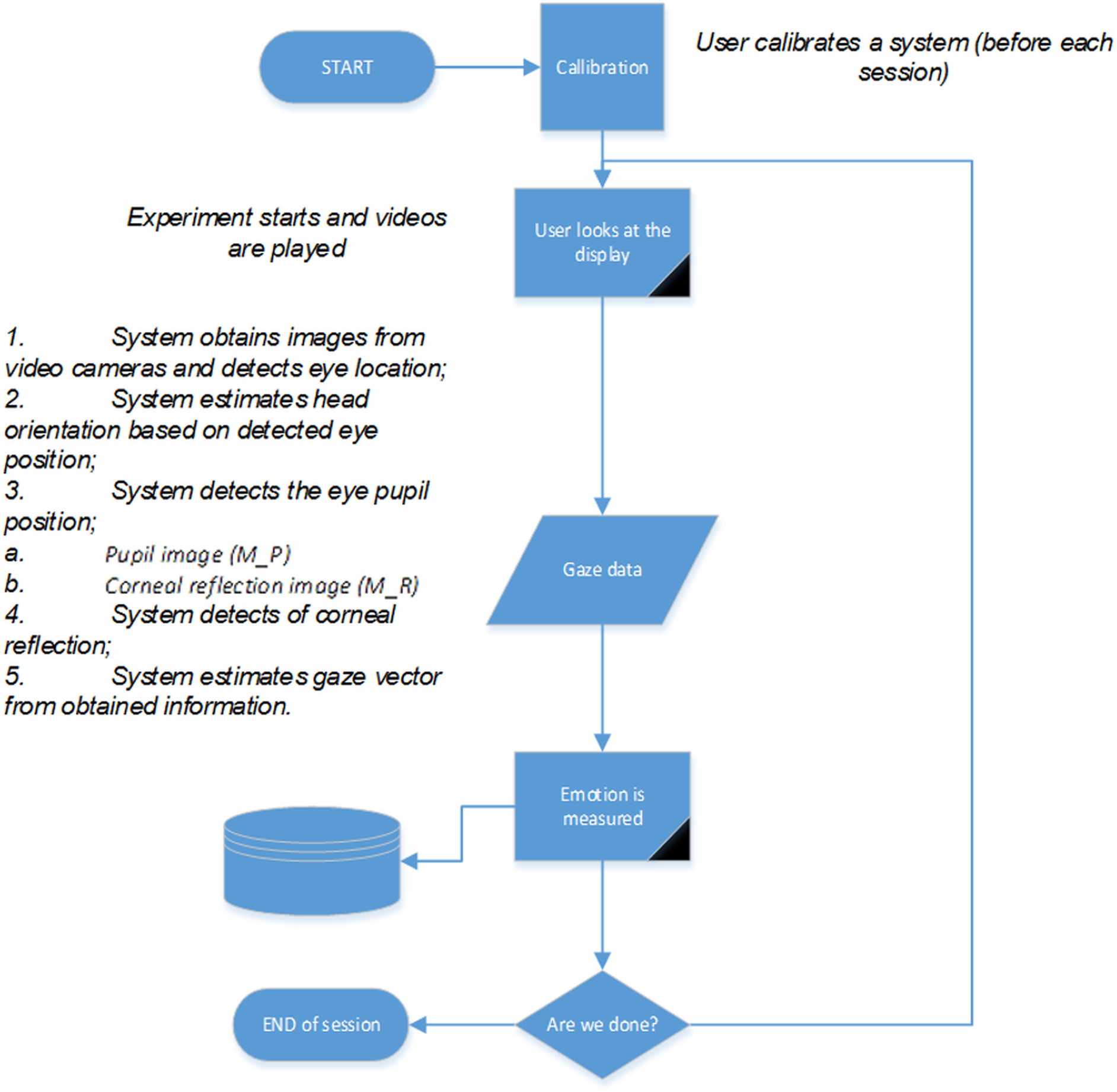
System workflow is illustrated in the flow chart shown in Fig. 5. Each participant was asked to calibrate the eye tracking system, based on a certain procedure. The chair was “fixed,” so the torso was not moving and the head position (gaze-point) on a turn back event remained stable. The orientation of the head was evaluated on the basis of the detected eye positions. The orientation angle was estimated between a horizontal line and a line drawn between the detected eye centers. Such an angle informs about how much a head is rotated around Y axis (inclined). All other rotation angles were controlled by not allowing additional movement (per instruction).
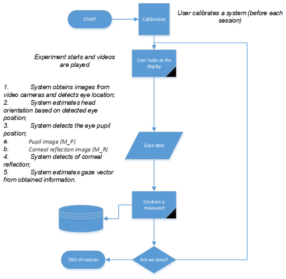
Figure 5: System workflow diagram.
Experimental Investigation
Experimental setup
Experiments were carried out during a day time, therefore a test room was illuminated mostly by a sun light only (amount and position changing over time) and, depending on the time of day, blinds were used on windows. Illumination levels were also impacted by door opening/closing (corridor is always brightly lit) during the early morning (∼8:00)/noon (∼17:00). The eye itself was illuminated using an infrared light source of eye tracker’s hardware. A difference vector between a pupil center and a glint point remained stable in most conditions. All data sets of a perceived session were reviewed manually. Data where our algorithm was unable to correct itself (missed an out of bounds event) was removed aiming not to impact results.
A total of 30 volunteers (20 males, 10 females, 24–42 years old) were asked to participate in testing the system of emotion recognition. We have chosen a similar set of participants as in our previous experiments (Raudonis et al., 2013; Raudonis, 2012). Unfortunately, a majority of people involved were not the same as two years have passed and we have had no opportunity to replicate that factor. To induce more reliable responses in participants, all experiments were conducted in an open-door environment (somebody often comes in) instead of a closed door laboratory type room as in our previous studies. An accidental visitor could observe a participant and experimental environment thus increasing the effect of stimuli, especially when content provoking shame and disgust emotions was demonstrated. Video materials (800*600) consisting of neutral, disgusting, shameful and “sensory pleasure” content (sample screenshots in Fig. 6) were played back in a close view on 24” 1080p monitor in full screen and with sound. All videos were gathered from the public domain with a help of psychologist. The database consists of five different clips (length 12 min each, 1 h total) for every emotion (total length of 4 h). Two out of those clips were used for training (24 min per emotion), other three (36 min per emotion) for evaluation. A randomly selected 2-minute fragment was displayed during training and evaluation stages, five times (two times during training, three times during evaluation) for each person per emotion (in total each person viewed 10 min of content (combined) per emotion). Videos used for training were not played during the evaluation. Each participant was given a 5-minute break between playback of different emotions. We have asked each participant to subjectively verify a perceived emotion and we have only used only “confirmed” signals. During a stimulation process the size of the pupil, the coordinates of the pupil center and a gaze point movement speed were registered.
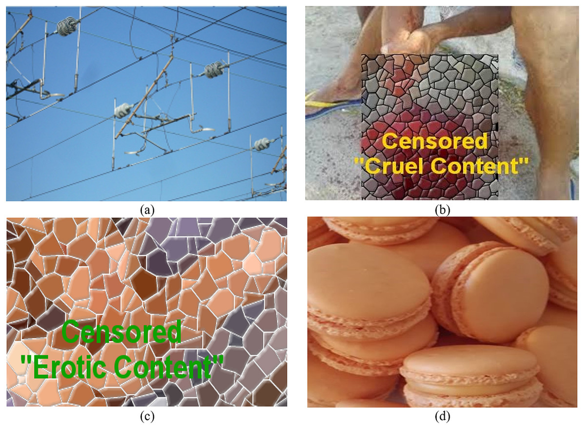
Figure 6: Visual stimulus samples which were used for experimental investigation and should invoke four different emotional states: (A) neutral, (B) disgust, (C) shame and (D) sensory pleasure.
Research on human subjects was approved by an Institutional Review Board of Kaunas University of Technology (document # 1409-16-04). 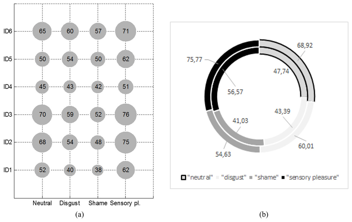
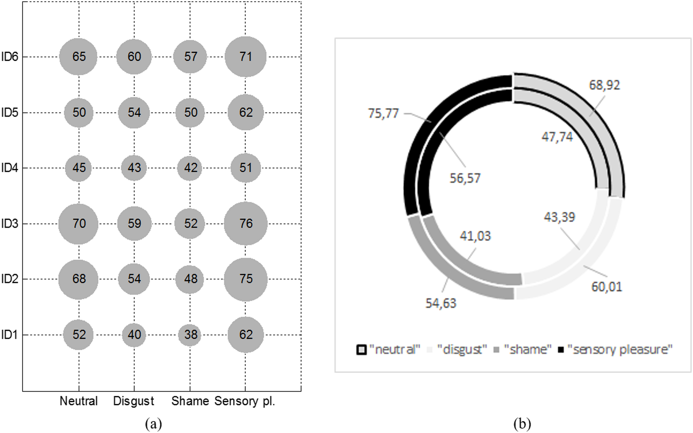
Figure 7: Average pupil size of first six participants who were stimulated with four different emotional stimuli (A) and average pupil size between participants of the experiment (B).
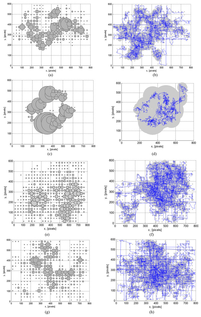
Figure 8: Attention map of ID1 participant (A, C, E, G) and average attention mapgaze trajectory (B, D, F, H) of all participants stimulated by the neutral (A and B), disgust (C and D), shameful (E and F) and “sensory pleasure” (G and H) emotional stimuli.
Experimental results
Figure 7A illustrates a sample fragment of measurements of the size of 6 people pupil. The size of each participant’s eye pupil was different during the perception process of each emotion, for example, the size of the first person’s pupil was ∼17 % larger when being in a neutral state vs being involved in a content (0.075 pixels vs 0.062 pixels). Deviation data have shown that it is important to note that the size can change significantly over time while likely still experiencing a similar emotion. This example proves that we cannot universally and subject-independently determine the real emotion a human was experiencing referring only to his eye pupil’s size. All remaining classification features have to be included.
Figure 7B illustrates an average pupil size for all of the participants (average of 30 people) who were stimulated with certain emotional stimuli. Red and blue lines mark variation limits of the pupil size. A pupil size shows that the highest emotional extremes were obtained when a person was stimulated by “sensory pleasure” and “shame” emotional stimuli.
Figure 8 illustrates attention concentration maps, representing attention map of the person stimulated with each specific emotion separately. The radius of each grey circle correlates with time spent to observe a specific part of the visual data and certain coordinates of the attention point. This is illustrated by the attention concentration map for one person on the left and the average attention map for all participants on the right. A blue line in the attention map represents a trajectory of the gaze point. Attention maps highlight different regions of two dimensional visual stimuli. Such distribution of attention points strongly depends on the felt emotion at a given moment. Attention maps are drawn with regard to presented visual data, arrangement of details in visual stimuli and cognitive capabilities of the individual person. Certain “parts” of the disgust emotional stimuli were ignored by all participants. A point of interest moves quite differently in a 2D space during each of the emotional stimuli. The next obvious conclusion was that this data might be usable to determine a current emotion. A movement parameter also depended on the context of emotional information shown on screen, as well as a position and motion of the object on screen (especially during videos where a view was concentrated on the specific subject). For example, all participants tried not to concentrate on the disgusting “bits” in videos, so an average trajectory covered a reasonably small path in 2D space. A large overlap of 2D space was noted when “sensory pleasure” videos for most of participants were played, as most viewed this content in a quite relaxed manner and did not concentrate much. When other types of materials were demonstrated, a movement was somewhat more concentrated. Playback of “shameful” (erotic movies) and to some extend “disgusting” content introduced a quick look “over the shoulder” effect (checking if someone was there to identify who is the public “sinner”—an effect which might very well be region and culture dependent). Smaller attention maps and longer trajectories were generated due to this effect (Figs. 8E–8F).
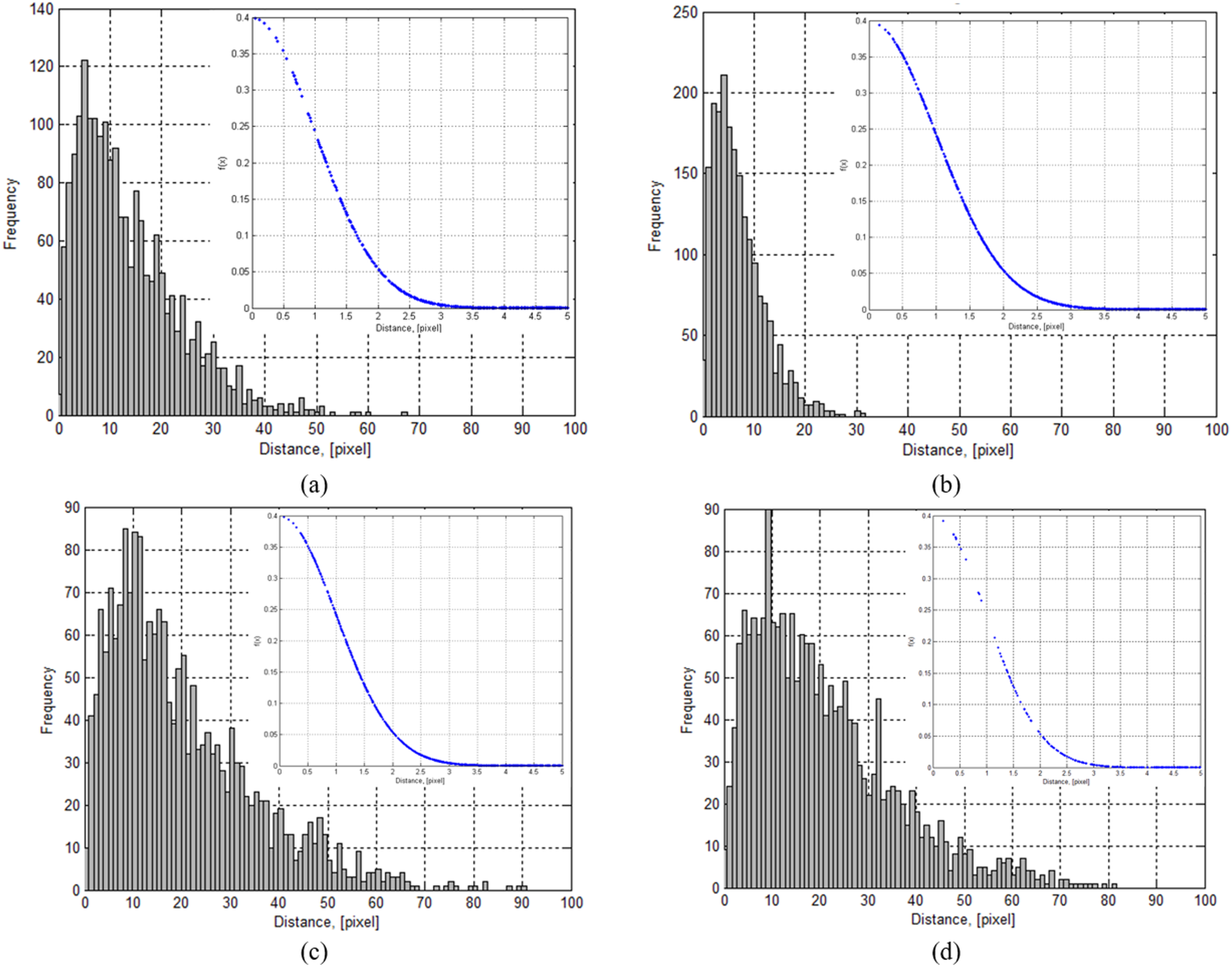
To evaluate a magnitude of changes in the trajectory of a gaze point, histograms and outcomes of a probability distance function (PDF) of distances between gaze fixation points and the speed of changing fixation points were given (Fig. 9). Data were calculated from the gaze trajectories acquired when participants were stimulated using (A) neutral, (B) disgust, (C) shameful and (D) “sensory pleasure” emotional stimuli. Pixel values were as calculated and were not rounded. PDFs were calculated using a standard MATLAB implementation (16). (16)
The first parameter μ is the mean. The second σ is the standard deviation.
| Emotion stimuli | Average jump distance (mean ± std), [pixels] |
|---|---|
| “Neutral” | 14.45 ± 20.7 |
| “Disgust” | 6.9 ± 4.9 |
| “Shame” | 36.7 ± 40.3 |
| “Sensory pleasure” | 23 ± 31.53 |
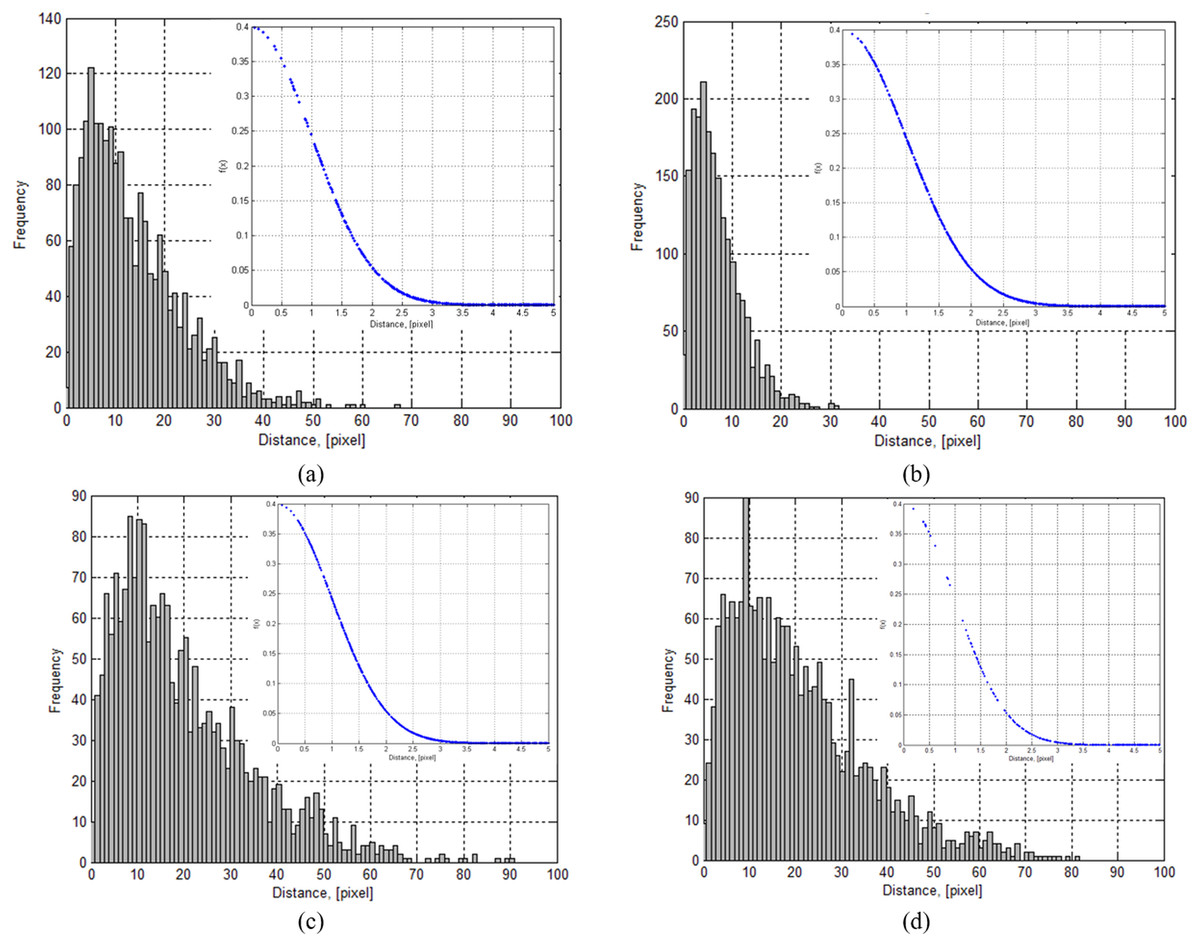
Figure 9: Average histogram and probability density function (top left corner) of distances between gaze fixation points when a person was stimulated with (A) neutral, (B) disgust, (C) shameful and (D) “sensory pleasure” emotional stimuli.
The average distance between gaze fixations points is given in Table 1. The smallest distance between gaze fixation points was estimated from a gaze trajectory when a person was stimulated with a disgust emotional stimulus. The highest jump in distance was generated when person was stimulated with a shameful emotional stimulus (part of a psychological effect of a person not wanting to be identified).
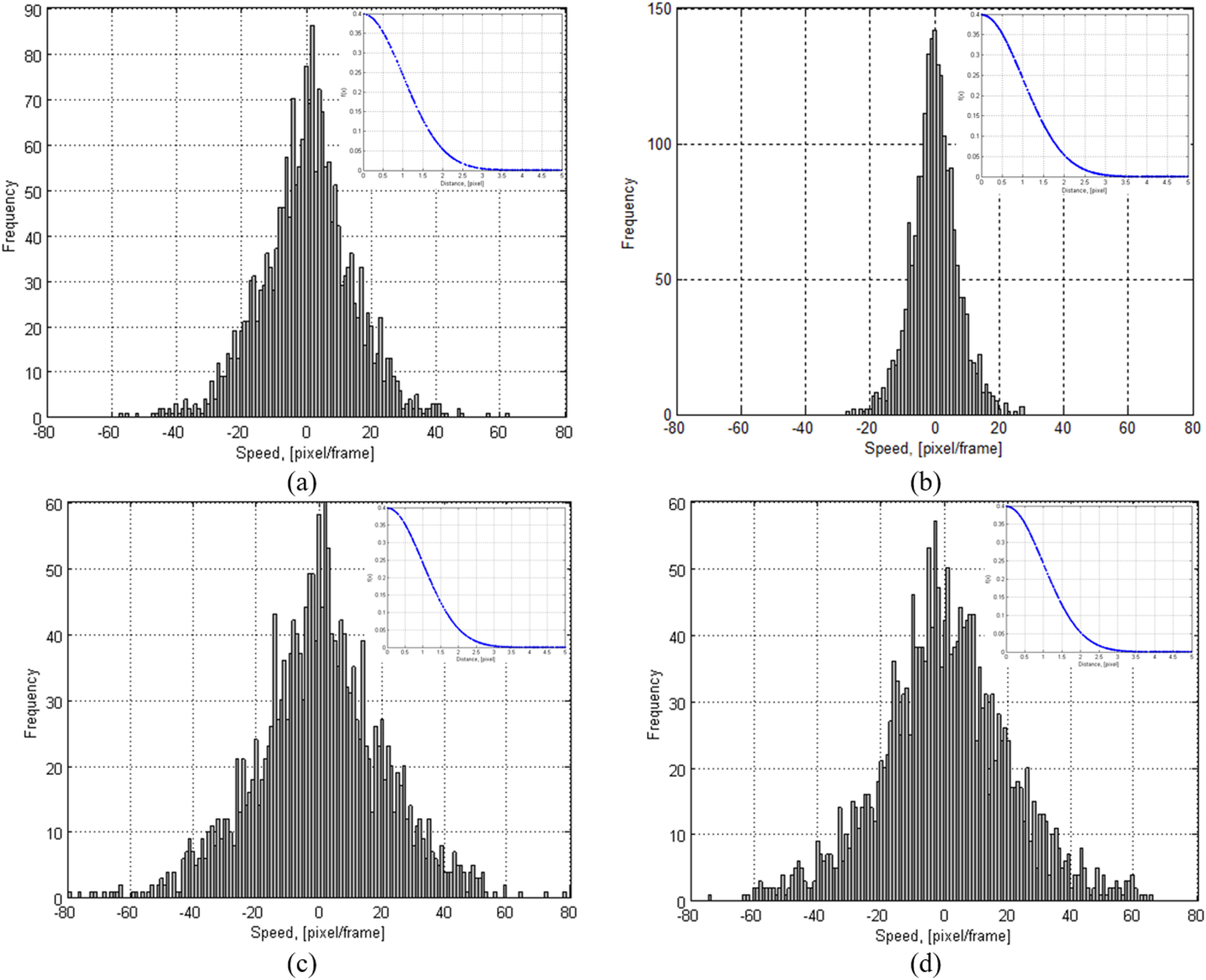
To evaluate the changes of speed in the trajectory of a gaze point, histograms and probability density functions of the gaze point change scale (speed of gazing) are shown in Fig. 10, representing a distribution of an average speed. The speed was evaluated with a pixel per frame value which showed how fast the gaze moved from frame to frame. Data were calculated from gaze trajectories when participants were stimulated using (a) neutral, (b) disgust, (c) shameful and (d) “sensory pleasure” emotional stimuli.
| Emotion stimuli | Average changes in speed (mean ± std), [pixels/frame] |
|---|---|
| “Neutral” | 0.011 ± 29.67 |
| “Disgust” | 0.0024 ± 7.02 |
| “Shameful” | 0.02 ± 57.10 |
| “Sensory pleasure” | −0.0021 ± 44.68 |
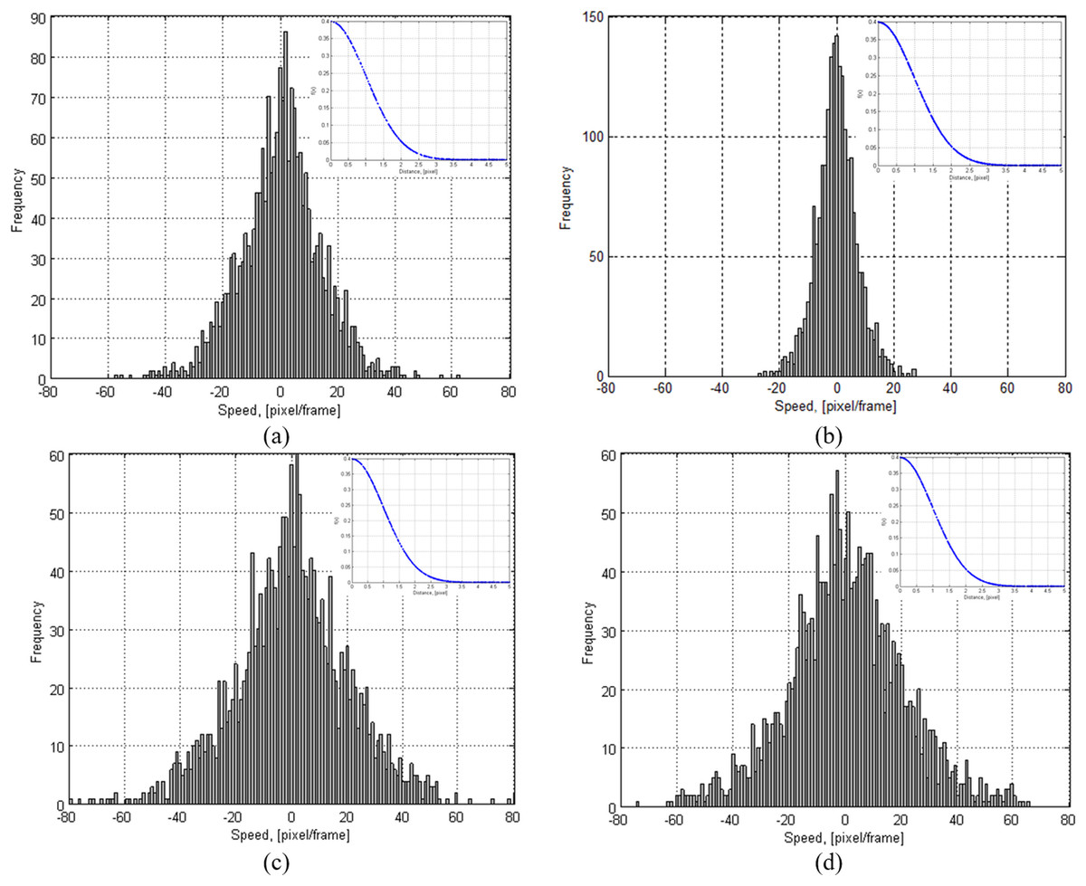
Figure 10: Average histogram and probability density function (top left corner) of changes in speed of a gaze point when a person was stimulated with (A) neutral, (B) disgust, (C) shameful and (D) “sensory pleasure” emotional stimuli.
Values of average changes of speed in the gaze trajectory are given in Table 2. Positive and negative values show a direction in which the gaze is moving. Therefore, a negative value of speed represents only a direction of gazing and how rapidly it changes. An average speed given varies around 0. This means that the gaze direction is rapidly changing around 0 (mu =0); therefore, the std value is more important here because it represents the distribution of speed. The speed is computed as location difference between frames F(t − 1) − F(t). The speed is defined as a simple sum of differences (see (16)). Positive and negative values show a direction in which the gaze is moving. Therefore, a negative value of speed represents only a direction of gazing and how rapidly it changes. The results showed that the smallest speed value was estimated from the gaze trajectory when a person was stimulated with disgusting emotional stimuli. The highest speed values were generated when a person was stimulated with shameful emotional stimuli. An average distribution in results of 30 people clearly illustrates that movement speeds were quite consistent and varied only during a playback of “shameful” content. The acceleration increased when our test subject experienced “strong” emotions or he was very interested in the information shown during the time-frame on a screen. Close to zero (0) value indicates that a person is focused for the moment (gaze does not move or the movement is minor). Negative and positive values are “fluctuations” to another point of interest on screen.
Table 3 illustrates an averaged confusion matrix (ACM) for all participants. The average classification accuracy is 0.85 and false positive is 0.04. Measured misclassification value was similar to every emotion.
| Emotion | “Neutral” | “Disgust” | “Shameful” | “Sensory pleasure” |
|---|---|---|---|---|
| “Neutral” | 0.85 | 0.03 | 0.07 | 0.05 |
| “Disgust” | 0.02 | 0.92 | 0.04 | 0.02 |
| “Shameful” | 0.05 | 0.05 | 0.82 | 0.08 |
| “Sensory pleasure” | 0.03 | 0.00 | 0.02 | 0.95 |

Figure 11: Relationship curves between classification accuracy and recorded samples used per classification feature (person dependent mode).
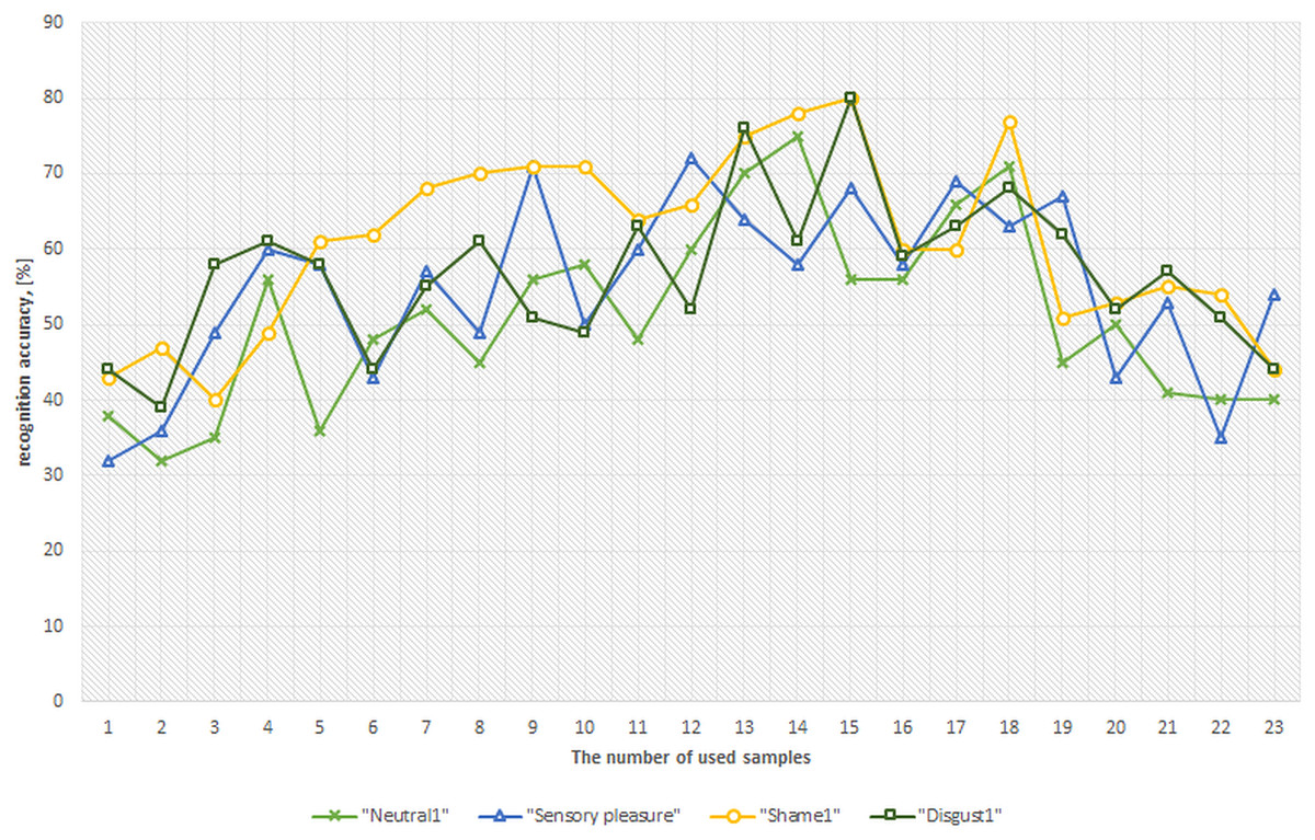
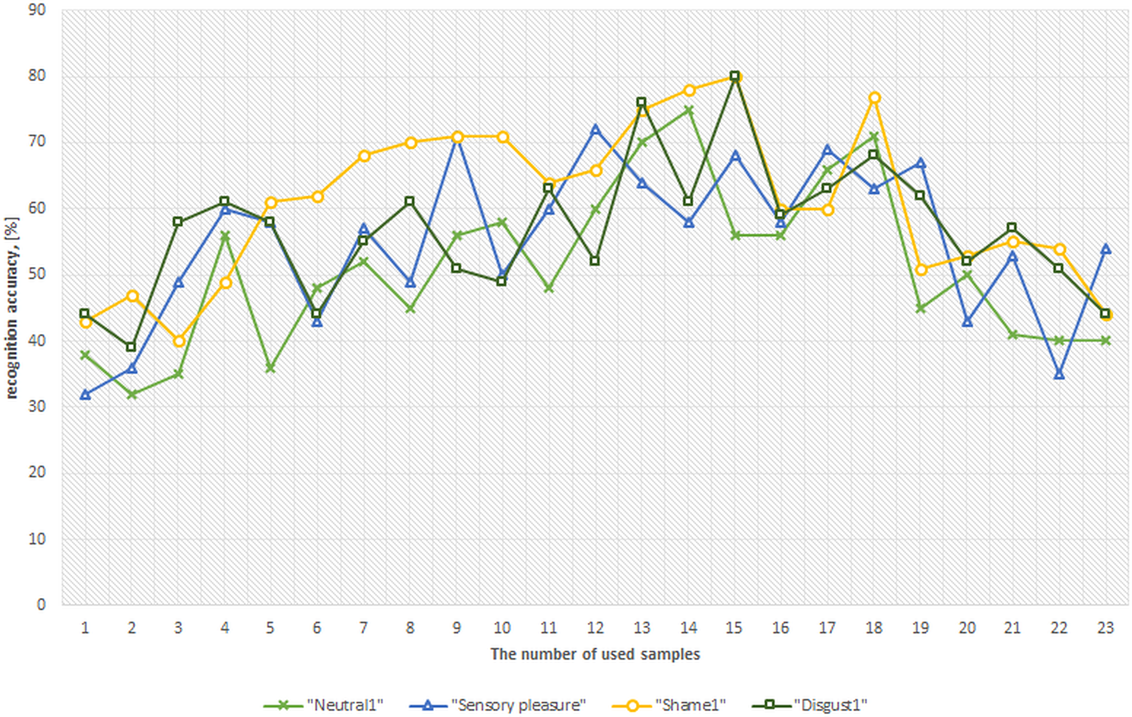
Figure 12: Relationship curves between classification accuracy and recorded samples used per classification feature (person independent mode).
Figure 11 illustrates the relationship between classification accuracy and a number of feature samples. A number of feature samples is represented on a horizontal axis and the achieved accuracy value is represented on a vertical axis. A curve of different colors represents different results of different emotional states. A total of 2 s of gaze “recordings” (approximately 17 samples on average) are necessary to achieve a 90 ± 3.5% recognition accuracy of a specific emotional state. Functional curves represent an average classification accuracy for all participants (combined). The largest changes in human’s visual mechanism that relay to an emotion are generated at the very beginning of emotional stimulation. The more samples we use (Frames * (d, x, y, v)), the more information we give to a NN which might not necessary accurately represent certain emotion.
Figure 12 shows person independent recognition performance, achieved by training ANN with emotional profiles of 10 people, and using the measured profiles of the remaining 20 persons for overall person-independent recognition accuracy evaluation. In a person independent mode, the best overall accuracy of 71.25 ± 5.1% was achieved using 13 samples and in comparison at 17 samples we have measured only 64.5 ± 4.2% overall recognition accuracy.
Discussion and Conclusion
The experiments have shown that each participant reacts differently to emotionally stimulating videos and the reaction or the emotional response strongly correlates with a cognitive perception, motivation and individual live experience of that person. Attention concentration maps proved to be very different for each visual stimulus. A certain person’s emotional state was recognized with a ∼90% of accuracy within an acceptable range of around 1 meter (eye-to-camera). Approximately 2 s (∼17 samples per feature) of measurements were needed to recognize a specific emotional state with a 10 ± 1.2% recognition error. The recognition error increased rapidly when fewer samples were used. “Disgust” emotional state was recognized with a highest recognition rate of 90.40 ± 3.5%. In this case, a clear distinction was noticed in a decreased (smaller than average) pupil’s size and a smaller distribution of the attention concentration maps. A “neutral” emotional state was recognized worst with a 13 ± 1.5% recognition error.
Compared to our previous works (Raudonis et al., 2013; Raudonis, 2012) where a close-to-eye gaze-tracker (mounted on glasses) and a comparable method of testing/algorithm was used, we have achieved a comparable result. Recognition accuracy also ranged in the interval from 80 to 90%, depending on a specific person and a certain emotion. A somewhat better recognition accuracy of the current remote eye tracker could also be contributed to an improved algorithm and (likely) to different hardware.
The future possibility of accurately determining an emotion without per-user gaze-tracker pre-calibration is very daunting (Wang, Wang & Ji, 2016; Alnajar et al., 2013). In a person independent mode we were able to achieve the best overall accuracy of 71.25 ± 5.1% using 13 samples. Ongoing investigation will naturally involve the rest of the main emotion group, and possibly other classification algorithms and methods. We are going to combine visual/audio stimuli with things you can touch and smell to better provoke the effect. We also aim at revisiting our previous experiments with a close-to-eye gaze-tracker to verify if renewed algorithms have had a noticeable effect on the overall recognition accuracy.