
Audio segmentation using Flattened Local Trimmed Range for ecological acoustic space analysis
- Published
- Accepted
- Received
- Academic Editor
- Abhishek Kumar
- Subject Areas
- Bioinformatics, Computational Biology
- Keywords
- Audio event detection, Flattened Local Trimmed Range, Bioacoustic
- Copyright
- © 2016 Vega et al.
- Licence
- This is an open access article distributed under the terms of the Creative Commons Attribution License, which permits unrestricted use, distribution, reproduction and adaptation in any medium and for any purpose provided that it is properly attributed. For attribution, the original author(s), title, publication source (PeerJ Computer Science) and either DOI or URL of the article must be cited.
- Cite this article
- 2016. Audio segmentation using Flattened Local Trimmed Range for ecological acoustic space analysis. PeerJ Computer Science 2:e70 https://doi.org/10.7717/peerj-cs.70
Abstract
The acoustic space in a given environment is filled with footprints arising from three processes: biophony, geophony and anthrophony. Bioacoustic research using passive acoustic sensors can result in thousands of recordings. An important component of processing these recordings is to automate signal detection. In this paper, we describe a new spectrogram-based approach for extracting individual audio events. Spectrogram-based audio event detection (AED) relies on separating the spectrogram into background (i.e., noise) and foreground (i.e., signal) classes using a threshold such as a global threshold, a per-band threshold, or one given by a classifier. These methods are either too sensitive to noise, designed for an individual species, or require prior training data. Our goal is to develop an algorithm that is not sensitive to noise, does not need any prior training data and works with any type of audio event. To do this, we propose: (1) a spectrogram filtering method, the Flattened Local Trimmed Range (FLTR) method, which models the spectrogram as a mixture of stationary and non-stationary energy processes and mitigates the effect of the stationary processes, and (2) an unsupervised algorithm that uses the filter to detect audio events. We measured the performance of the algorithm using a set of six thoroughly validated audio recordings and obtained a sensitivity of 94% and a positive predictive value of 89%. These sensitivity and positive predictive values are very high, given that the validated recordings are diverse and obtained from field conditions. The algorithm was then used to extract audio events in three datasets. Features of these audio events were plotted and showed the unique aspects of the three acoustic communities.
Introduction
The acoustic space in a given environment is filled with footprints of activity. These footprints arise as events in the acoustic space from three processes: biophony, or the sound species make (e.g., calls, stridulation); geophony, or the sound made by different earth processes (e.g., rain, wind); and anthrophony, or the sounds that arise from human activity (e.g., automobile or airplane traffic) (Krause, 2008). The field of Soundscape Ecology is tasked with understanding and measuring the relation between these processes and their acoustic footprints, as well as the total composition of this acoustic space (Pijanowski et al., 2011). Acoustic environment research depends more and more on data acquired through passive sensors (Blumstein et al., 2011; Aide et al., 2013) because recorders can acquire more data than is possible manually (Parker III, 1991; Catchpole & Slater, 2003; Remsen, 1994), and these data provide better results than traditional methods (Celis-Murillo, Deppe & Ward, 2012; Marques et al., 2013).
Currently, most soundscape analysis focus on computing indices for each recording in a given dataset (Towsey et al., 2014), or on plotting and aggregating the raw acoustic energy (Gage & Axel, 2014). An alternative approach is to use each individual acoustic event as the base data and aggregate features computed from these events, but up until now, it has been difficult to accurately extract individual acoustic events from recordings.
We define an acoustic event as a perceptual difference in the audio signal that is indicative of some activity. While being a subjective definition, this perceptual difference can be reflected in transformations of the signal (e.g., a dark spot in a recording’s spectrogram).
Normally, to use individual acoustic events as base data, a manual acoustic event extraction is performed (Acevedo et al., 2009). This is usually done as a first step to build species classifiers, and can be made very accurately. By using an audio visualization and annotation tool, an expert is able to draw a boundary around an acoustic event; however, this method is very time-consuming, is specific to a set of acoustic events and it is not easily scalable for large datasets (e.g., >1000 minutes of recorded audio), thus an automated detection method could be very useful.
Acoustic event detection (AED) has been used as a first step to build species classifiers for whales, birds and amphibians (Popescu et al., 2013; Neal et al., 2011; Aide et al., 2013). Most AED approaches rely on using some sort of thresholding to binarize the spectrogram into background (i.e., noise) and foreground (i.e., signal) classes. Foreground spectrogram cells satisfying some contiguity constraint are then joined into a single acoustic event. Some methods use a global threshold (Popescu et al., 2013), or a per-band threshold (Brandes, Naskrecki & Figueroa, 2006; Aide et al., 2013), while others train a species-specific classifier to perform the thresholding (Neal et al., 2011; Briggs, Raich & Fern, 2009). In Towsey et al. (2012) the authors reduce the noise in the spectrogram by using a 2D Wiener filter and removing modal intensity on each frequency band before applying a global threshold, but the threshold and parameters used in the AED tended to be species specific. Rather than using a threshold approach, Briggs et al. (2012) trained a classifier to label each cell in the spectrogram as sound or noise. These methods are either too sensitive to noise, are specialized to specific species, require prior training data or require prior knowledge from the user. What is needed is an algorithm that works for any recording, is not targeted to a specific type of acoustic event, does not need any prior training data, is not sensitive to noise, is fast and requires as little user intervention as possible.
In this article we propose a spectrogram filtering method, the Flattened Local Trimmed Range (FLTR) method, and an unsupervised algorithm that uses this filter for detecting acoustic events. This method filters the spectrogram by modeling it as a mixture of stationary and non-stationary energy processes, and mitigates the effect of the stationary processes. The detection algorithm applies FLTR to the spectrogram and proceeds to threshold it globally. Afterward, each contiguous region above the threshold line is considered an individual acoustic event.
We are interested in detecting automatically all acoustic events in a set of recordings. As such, this method tries to remove all specificity by design. Because of this, this method can work as a form of data reduction. As a first step, this transforms the acoustic data into a set of events that can later feed further analysis.
The presentation of the article follows the workflow in Fig. 1: given a set of recordings, we compute the spectrogram for each one, then the FLTR is computed, a global threshold is applied and, finally, we proceed to extract the acoustic events. These acoustic events are compared with manually labeled acoustic events to determine the precision and accuracy of the automated process. We then applied the AED methodology to recordings from three different sites. Features of the events were calculated and plotted to determine unique aspects of each site. Finally, events within a region of high acoustic activity were sampled to determine the sources of these sounds.
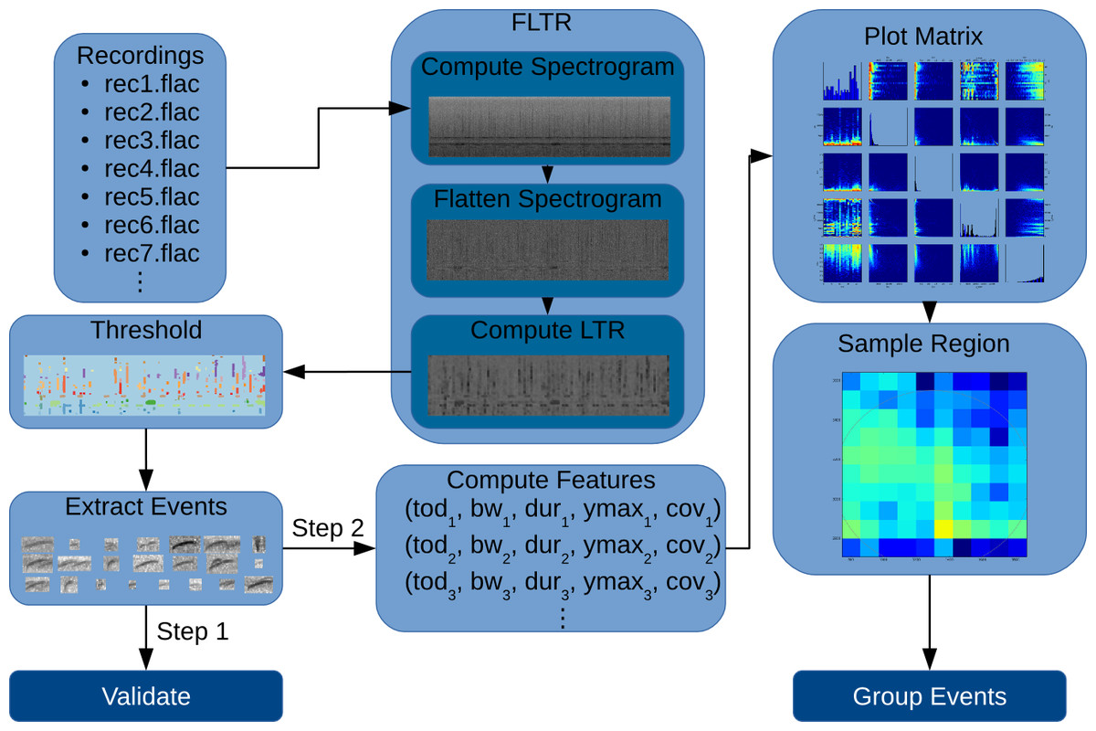
Figure 1: Flow diagram showing the workflow followed in this article.
Recordings are filtered using FLTR, then thresholded. Contiguous cells form each acoustic event. In step 1, we validate the extracted events. In step 2, we compute features for each event and plot them. Acoustic events from one of the plotted regions are then sampled and cataloged.
Theory
Audio spectrogram
The spectrogram of an audio recording separates the power in the signal into frequency components in a short time window along a much longer time dimension (Fig. 2A). The spectrogram is defined as the magnitude component of a Short Time Fourier Transform (STFT) on the audio data and it can be viewed as a time-frequency representation of the magnitude of the acoustic energy. This energy gets spread over distinct frequency bins as it changes over time. Thus, providing a way of analyzing audio not just as a linear sequence of samples, but as an evolving distribution, where each acoustic event is rendered as high energy magnitudes in both time and frequency.
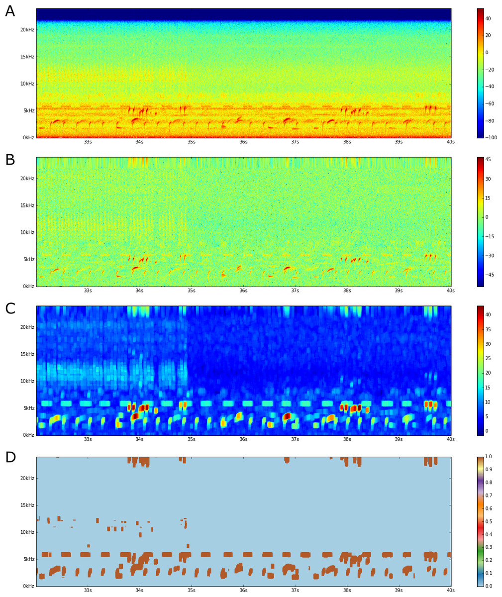
Figure 2: FLTR steps.
(A) An audio spectrogram. Color scale is in dB. (B) A band flattened spectrogram. (C) Local Trimmed Range (20 × 20 window). (D) Thresholded image.
We represent a given spectrogram as a function S(t, f), where 0 ≤ t < τ and 0 ≤ t < η are the time and frequency coordinates, bounded by τ, the number of audio frames given by the STFT and η, the number of frequency bins in the transform.
The Flattened Local Trimmed Range
The first step in detecting acoustic events in the spectrogram requires creating the Flattened Local Trimmed Range (FLTR) image. Once we have the spectrogram, creating the FLTR requires two steps: (1) flattening the spectrogram and (2) computing the local trimmed range (Figs. 2B–2C). This image is produced by modeling the spectrogram as a sum of different energetic processes, along with some assumptions on the distributions of the acoustic events, and a proposed solution that takes advantage of the model to separate the energetic processes.
Modeling the spectrogram
We model the spectrogram Sdb(t, f) as a sum of different energetic processes: (1) where b(f) is a frequency-dependent process that is taken as constant in time, while ϵ(t, f) is a process that is stationary in time and frequency with 0-mean, 0-median, and some scale parameter, and Ri(t, f) is a set of non-zero-mean localized energy processes that are bounded by their support functions , for 1 ≤ i ≤ n. An interpretation for these energetic processes is that b(f) corresponds to a frequency-dependent near-constant noise, ϵ(t, f) corresponds to a global noise process with a symmetric distribution and the Ri(t, f) are our acoustic events, of which there are n.
In this model, we assume that the set of localized energy processes has four properties:
-
A1
The localized energy processes are mutually exclusive and are not adjacent. That is, no two localized energy processes share in the same (t, f) coordinate, nor do they have adjacent coordinates. Thus, ∀1 ≤ i, j ≤ n, i ≠ j, 0 ≤ t < τ, 0 ≤ f < η, we have:
This can be done without loss of generality. If two such localized processes existed, we can just consider their union as one.
-
A2
The regions of localized energy processes dominate the energy distribution in the spectrogram on each given band. That is, ∀0 ≤ t1, t2 < τ, 0 ≤ f < η, we have:
-
A3
The proportion of samples within a localized energy processes in a given frequency band, denoted as ρ(f), is less than half the samples in the entire frequency band. That is, ∀0 ≤ f < η, we have:
-
A4
Each localized energy process dominates the energy distribution in its surrounding region, when accounting for frequency band-dependent effects. That is, for every (t1, f1) point that falls inside a localized energy process (∀1 ≤ i ≤ n, 0 ≤ t1 < τ, 0 ≤ f1 < η) where ), there is a region-dependent time-based radius ri,1 and a frequency-based radius ri,2, such that for every other (t2, f2) point around the vicinity (∀(t2, f2) ∈ [t1 − ri,1, t1 + ri,1] × [f1 − ri,2, f1 + ri,2]), we have:
We want to extract the Ri components or, more specifically, their support functions , from the spectrogram. If we are able to estimate b(f) reliably for a given spectrogram, we can then compute , a spectrogram that is corrected for frequency intensity variations. Once that is done, we compute local statistics to estimate the regions and, thus, segregate the spectrogram into the localized energy processes Ri(t, f) and an ϵ(t, f) background process.
Flattening—estimating b(f)
Other than A2, A3 and A4, we do not hold any assumptions for ϵ(t, f) or Ri(t, f). In particular we do not presume to know their distributions. Thus, it is difficult to formulate a model to compute a Maximum A-Posteriori Estimator of b(f)|Sdb(t, f). Even so, the frequency sample means of a given spectrogram do not give a good estimate on b(f) since they get mixed with the sum of non-zero expectations of any intersecting region:
Since ϵ(t, f) is a stationary 0-mean process, we do not need to worry about it as it will eventually cancel itself out, but the localized energy process regions do not cancel out. Since our goal is to separate these regions from the rest of the spectrogram in a general manner, if an estimate of b(f) is to be useful, it should not depend on the particular values within these regions.
While using the mean does not prove to be useful, we can use the frequency sample medians, along with A2 and A3 to remove any frequency-dependent time-constant bands from the spectrogram. We formalize this with the following theorem:
Let 0 ≤ f ≤ η be a frequency band in the spectrogram, with a proportion of localized energy processes given as , and a median m(f). Assume A2 and that ρ(f) < .5, then m(f) depends only in the ϵ process and does not depend on any of the localized energy processes Ri(t, f).
ρ(f) is the proportion of energy samples in a given frequency band f that participate in a localized energy process. Then, ρ(f) < .5 implies that less than 50% of the energy samples do so. This means that a 1 − ρ(f) > .5 proportion of the samples in band f are described by the equation Sdb(t, f) = b(f) + ϵ(t, f). A2 implies that the lower half of the population is within this 1 − ρ(f) proportion, along with the frequency band median m(f). Thus m(f) does not depend on the localized energy processes Ri(t, f). □
Thus, assuming A2 and A3, m(f) gives an estimator whose bias is limited by the range of the ϵ process and is completely unaffected by the Ri processes. Furthermore, as ρ(f) approaches 0, m(f) approaches b(f).
We use the term band flattening to refer to the process of subtracting the b(f) component from Sdb(t, f). Thus we call the band flattened spectrogram estimate of Sdb(t, f). Figure 2B shows the output from this flattening procedure. As can be seen, this procedure removes any frequency-dependent time-constant bands in the spectrogram.
Estimating
We can use the band flattened spectrogram to further estimate the regions, since:
We do this by computing the local α-trimmed range . That is, given some 0 ≤ α < 50, and some r > 0, for each (t, f) pair, we compute: where Pα(⋅) is the α percentile statistic, and is the band flattened spectrogram, with its domain restricted to a square neighborhood of range r (in time and frequency) around the point (t, f).
Assuming A4, the estimator would give small values for neighborhoods without localized energy processes, but would peak around the borders of any such process. This statistic could then be thresholded to compute estimates of these borders and an estimate of the support functions . Figure 2C shows the local trimmed range of a flattened spectrogram image. As can be seen, areas with acoustic events have a higher local trimmed range, while empty areas have a lower one.
Thresholding
There are many methods that can be used to threshold the resulting FLTR image (Sezgin & Sankur, 2004). Of these, we use the entropy-based method developed by Yen, Chang & Chang (1995). This method works on the distribution of the values, it defines an entropic correlation TC(t) of foreground and background classes as: where m and M are the minimum and maximum values of the FLTR spectrogram, and f(⋅) and F(⋅) are the Probability Density Function (PDF) and Cumulative Density Function (CDF) of these values. The PDF and CDF, in this case, are approximated with a histogram. The Yen threshold is then the value that maximizes this entropy correlation. That is: Figure 2D shows a thresholded FLTR image of a spectrogram. Adjacent (t, f) coordinates whose value is greater than the threshold are then considered as the border of one acoustic event. The region enclosed by such borders, including the borders, are then the acoustic events detected within the spectrogram.
Data and Methodology
Data
To test the FLTR algorithm we used two datasets collected and stored by the ARBIMON system (Sieve Analytics, 2015; Aide et al., 2013). The recordings were captured using passive audio recording equipment from different locations as part of a long-term audio monitoring network.
The first dataset, the validation dataset, consisted of 2,051 manually labeled acoustic events from six audio recordings (every acoustic event was labeled) (validation data, https://dx.doi.org/10.6084/m9.figshare.2066028.v1). This set includes a recording from Lagoa do Peri, Brazil; one recording from the Arakaeri Communal Reserve, Perú; one from El Yunque, Puerto Rico; and three underwater recordings from Mona Island, Puerto Rico.
The second dataset, the sites dataset, was a set of 240 recordings from the Amarakaeri Communal Reserve in Perú (from June 2014 to February 2015), 240 recordings from El Verde area in El Yunque National Forest, Puerto Rico (from March 2008 to July 2014), and 240 recordings from a wetland in Sabana Seca, Puerto Rico (from March 2008 to August 2014) (Amarakaeri Perú recordings, https://dx.doi.org/10.6084/m9.figshare.2065419.v2; El Verde recordings, https://dx.doi.org/10.6084/m9.figshare.2065908.v1; Sabana Seca recordings, https://dx.doi.org/10.6084/m9.figshare.2065929.v1). Each set consisted of 10 one-minute recordings per hour, for all 24 h, sampled uniformly from larger datasets from each site.
Methodology
We divided our methodology into two main steps. In the first step, FLTR validation, we extracted acoustic events from the recordings in the first dataset, which we then validated against the manually labeled acoustic events. In the second step, site acoustic event visualization, we extracted the acoustic events from the second dataset, computed feature vectors for each event and plotted them. The recording spectrograms were computed using a Hann window function of 512 audio samples and an overlap of 256 samples.
FLTR validation
We used the FLTR algorithm with a 21 × 21 window and α = 5 to extract the acoustic events and compared them with the manually labeled acoustic events.
For the validation, we used two comparison methods, the first is based on a basic intersection test between the automatically detected and the manually labeled events’ bounds, and the second one is based on an overlap percent. For each manual label and detection event pair, we defined the computed overlap percent as the ratio of the area of their intersection and the area of their union: where L is a manually labeled event, D is a automatically detected event area, and and are the area of the intersection and the union of their respective bounds.
On the first comparison method, for each acoustic event whose bounds intersected the bounds of a manually labeled acoustic event, we registered it as a detected acoustic event. For each detected event whose bounds did not intersect any manually labeled acoustic events, we registered it as detected, but without an acoustic event. On the other hand, the manually labeled acoustic events that did not intersect any detected acoustic event were registered as undetected acoustic events.
The second method followed a similar path as the first, but it requires an overlap percent of at least 25%. For each acoustic event whose overlap percent with a manually labeled acoustic event was greater than or equal to 25%, we registered it as a detected acoustic event. For each detected event that did not have any manually labeled acoustic events with an overlap percent of at least 25%, we registered it as detected, but without an acoustic event. On the other hand, the manually labeled acoustic events that did not have an overlap percent of at least 25% with any detected acoustic event were registered as undetected acoustic events.
These data were used to create a confusion matrix to compute the FLTR algorithm’s sensitivity and positive predictive value for each method. The sensitivity is computed as the ratio of the number of manually labeled acoustic events that were automatically detected (true positives) over the total count of manually labeled acoustic events (true positives and false negatives). This measurement reflects the percent of detected acoustic events that were present in the recording.
The positive predictive value is computed as the ratio of the number of manually labeled acoustic events that were automatically detected (true positives) over the total count of detected acoustic events (true positives and false positives). This measurement reflects the percent of real acoustic events among the set of detected acoustic events.
FLTR application
As with the FLTR validation step, we used the FLTR algorithm with a 21 × 21 window and α = 5 to extract the acoustic events in each of the recording samples in the second dataset, which we then converted into feature vectors.
The variables computed for each extracted acoustic event Ri were:
-
Time of Day. Hour in which the recording from this acoustic event was taken.
-
Bandwidth. Length of the acoustic event in Hertz. That is, given , the bandwidth is defined as: (2)
-
Duration. Length of the acoustic event in seconds. That is, given , the duration is defined as: (3)
-
Dominant Frequency. The frequency at which the acoustic event attains its maximum power: (4)
-
Coverage Ratio. The ratio between the area covered by the detected acoustic event and the area detected by the bounds: (5)
Using these features, we generate a log-density plot matrix for all pairwise combinations of the features for each site. The plots in the diagonal are log histograms of the column feature.
We measured the information content of each feature pair by computing their joint entropy H: where log2 is the base 2 logarithm, hi,j is the number of events in the (i, j)th bin of the joint histogram, and N1 and N2 are the number of bins of each variable in the histogram. A higher value of H means a higher information content.
We also focused our attention on areas with a high and medium count of detected acoustic events (log of detected events greater than 6 and 3.5, respectively). As an example, we selected an area of interest in the feature space of the Sabana Seca dataset (i.e., a visual cluster in the bw vs. y˙max plot). We sampled 50 detected acoustic events from the area and categorized them manually.
Results
FLTR validation
Under the simple intersection test, out of 2,051 manually labeled acoustic events, 1,922 were detected (true positives), and 129 were not (Table 1). Of the 2,167 detected acoustic events, 1,922 were associated with manually labeled acoustic events (true positives), and 245 were not (false negatives). This resulted in a sensitivity of 94% and a positive predictive value of 89%.
| Acoustic event | No acoustic event | Total | |
|---|---|---|---|
| Detected | 1,922 | 245 | 2,167 |
| Not detected | 129 | – | 129 |
| Total | 2,051 | 245 | 2,296 |
| Sensitivity | 1,922/2,051 | 94% |
| Positive predictive value | 1,922/2,167 | 89% |
Under the overlap percentage test, out of 2,051 manually labeled acoustic events, 1,744 were detected (true positives), and 307 were not (Table 2). Of the 2,167 detected acoustic events, 1,744 were associated with manually labeled acoustic events (true positives), and 423 were not (false negatives). This resulted in a sensitivity of 85% and a positive predictive value of 80%.
Figure 3 shows the spectrograms of a sample of six acoustic events from the validation step, along with their FLTR images. Figures 3A–3D are manually labeled acoustic events that were detected. Figures 3E–3H are manually labeled acoustic events that were not detected. Figures 3I–3L are detected acoustic events that were not labeled. The FLTR images show how the surrounding background gets filtered and the acoustic event stands above it. Figures 3F shows lower than threshold FLTR values, possibly due to the spectrogram flattening. FLTR values in Fig. 3H is too low to cross the threshold as well and Fig. 3I shows a detection of some low-frequency short lived audio noise.
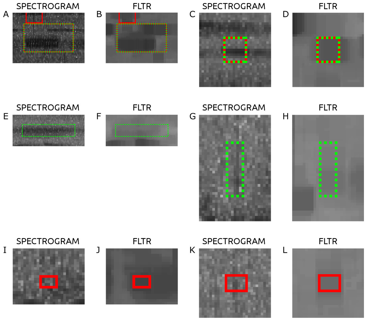
Figure 3: Sample of the intersections of 6 acoustic events along with their FLTR image.
(A–D) are manually labeled and detected, (E–H) are manually labeled but not detected detected, and (I–L) are detected but not manually labeled.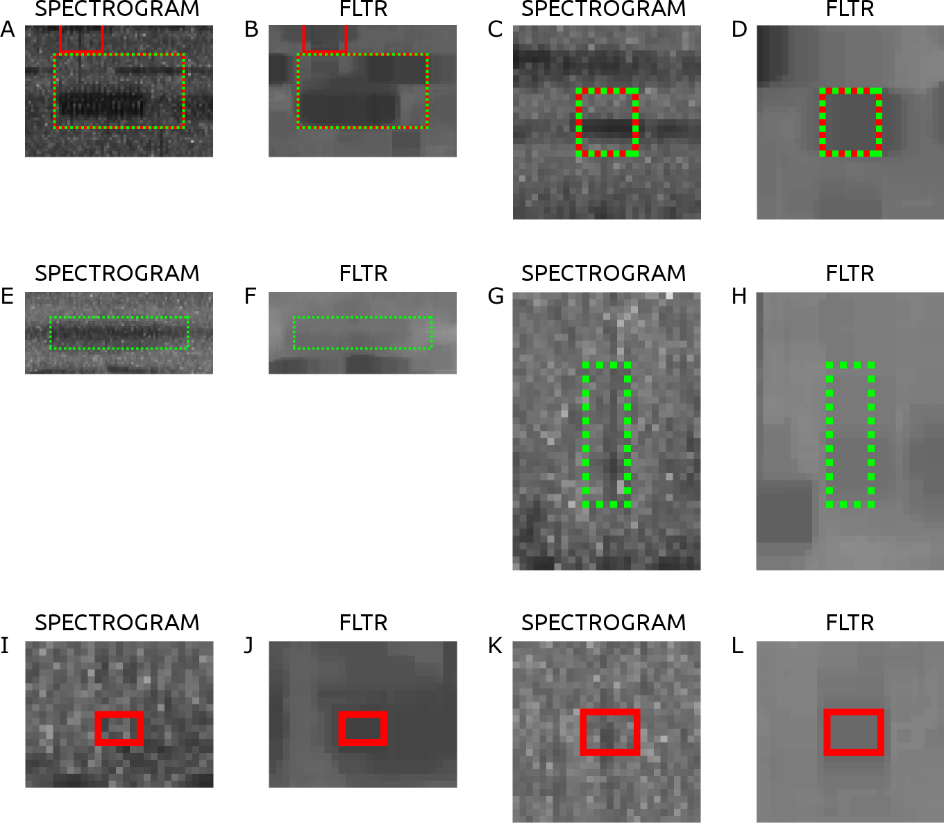
| Acoustic event | No acoustic event | Total | |
|---|---|---|---|
| Detected | 1,744 | 423 | 2,167 |
| Not detected | 307 | — | 307 |
| Total | 2,051 | 423 | 2,296 |
| Sensitivity | 1,744/2,051 | 85% |
| Positive predictive value | 1,744/2,167 | 80% |
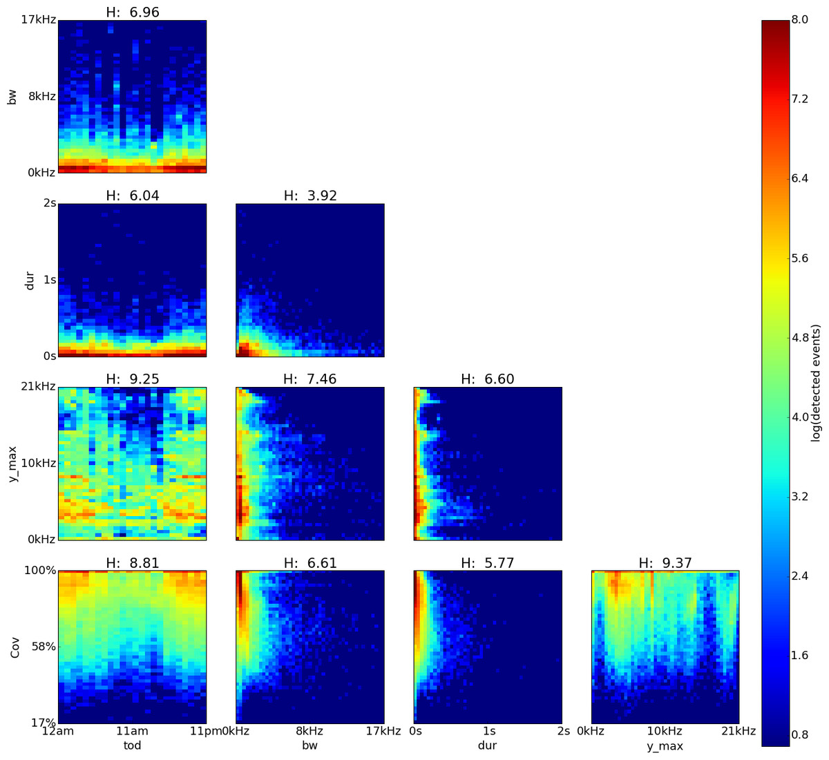
Figure 4: Amarakaeri, Perú, log density plot matrix of acoustic events extracted from 240 sample recordings.
Variables shown are time of day (tod), bandwidth (bw), duration (dur), dominant frequency (y˙max) and coverage (cov). Note high H values for cov vs. y˙max (9.37), y˙max vs. tod (9.25) and cov vs. tod(8.81) .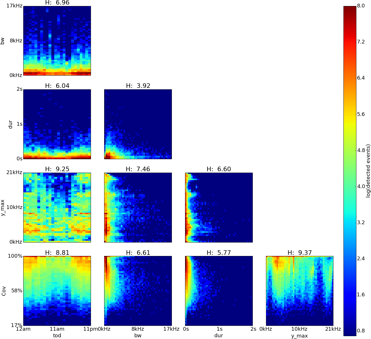
FLTR application
The feature pairs with highest joint entropy in the plots of the Perú recordings are cov vs. y˙max, y˙max vs. tod and cov vs. tod with values of 9.37, 9.25 and 8.81 respectively (Fig. 4). The cov vs. y˙max plot shows three areas of high event detection count at 2.4–4.6 kHz with 84–100% coverage, 7.0–7.4 kHz with 88–100% coverage and 8.4–8.8 kHz with 84–100% coverage. Three areas of medium event detection count can be found at 12.8–14.9 kHz with 68–90% coverage, 18.5–20.4 kHz with 59–90% coverage and one spanning the whole 90–100% coverage band. The y˙max vs. tod plot shows two areas of high event detection count from 5pm to 5am at 2.9–5.9 kHz and from 7pm to 4am at 9.6–10 kHz. Three areas of medium event detection count can be found at from 6pm to 5am at 17.6–20.9 kHz, from 5pm to 5am at 15.7–10.5 kHz and one spanning the entire day at 7.5–10.5 kHz. The cov vs. tod plot shows one area of high event detection count from 6pm to 5am with 84–100% coverage and another area of medium event detection count throughout the entire day with 60–84% coverage from 6pm to 5am and with 77–100% coverage from 6am to 5pm.
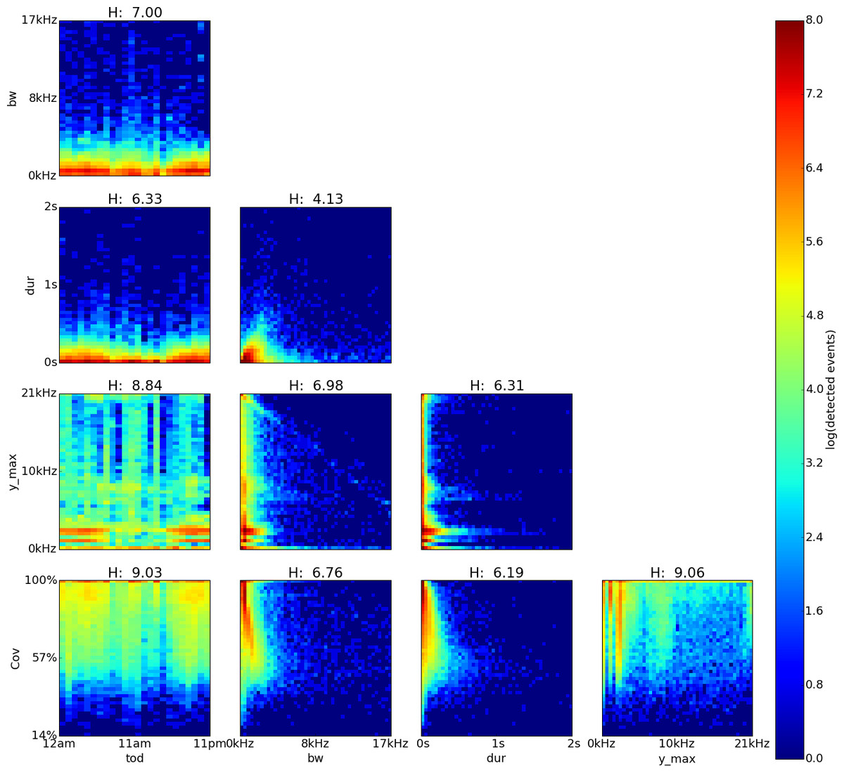
Figure 5: El Verde, Puerto Rico, log density plot matrix of acoustic events extracted from 240 sample recordings.
Variables shown are time of day (tod), bandwidth (bw), duration (dur), dominant frequency (y˙max) and coverage (cov). Note high Hn values for tod (0.98), cov (0.84) and y˙max (0.83).
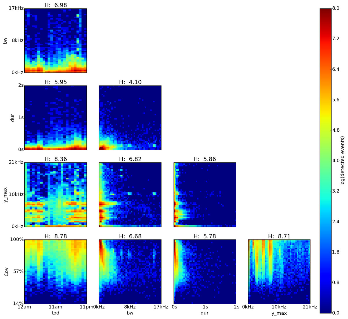
Figure 6: Sabana Seca, Puerto Rico, log density plot matrix of audio events extracted from 240 sample recordings.
Variables shown are time of day (tod), bandwidth (bw), duration (dur), dominant frequency (y˙max) and coverage (cov). Note high Hn values for tod (0.96), cov (0.81) and y˙max (0.8).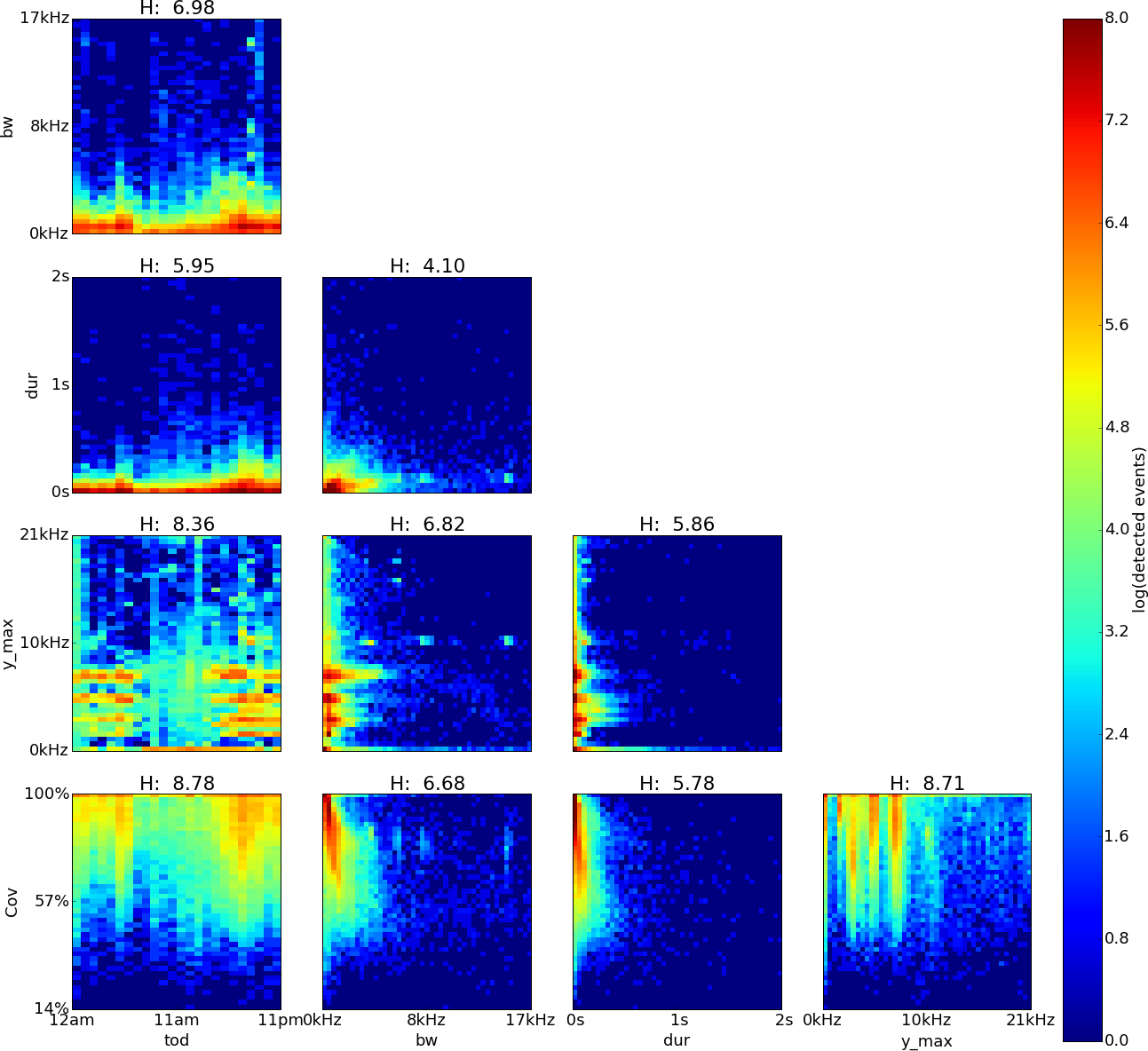
The feature pairs with highest joint entropy in the plots of the El Verde recordings are cov vs. y˙max, y˙max vs. tod and cov vs. tod with values of 9.06, 9.03 and 8.84 respectively (Fig. 5). The cov vs. y˙max plot shows two areas of high event detection count at 3.3–1.9 kHz with 67–100% coverage and 1.4–0.8 kHz with 82–100% coverage. Three areas of medium event detection count can be found at 7.1–9.8 kHz with 59–98% coverage, 20.1–20.8 kHz with 65–98% coverage and one spanning the whole 98–100% coverage band. The y˙max vs. tod plot shows three areas of high event detection count from 6pm to 7am at 1.9–2.9 kHz, from 7pm to 6am at 1.0–1.4 kHz and one spanning the entire day at 0–0.5 kHz. Two areas of medium event detection count span the whole day, one at 3.5–5.1 kHz and another one at 6.1–9.9 kHz. Vertical bands of medium event detection count areas can be found at 12am–5am, 7am, 10am–12pm, 3pm and 8pm. The cov vs. tod plot shows an area of medium event detection count spanning the entire day with 46–100% coverage, changing to 75–100% coverage from 1pm to 5pm. There seems to be a downward trending density line on the upper left corner of the plot in y˙max vs. bw.
The feature pairs with highest joint entropy in the plots of the Sabana Seca recordings are cov vs. y˙max, y˙max vs. tod and cov vs. tod with values of 8.71, 8.78 and 8.36 respectively (Fig. 6). The cov vs. y˙max plot shows four areas of high event detection count at 0–0.2 kHz with 83–100% coverage, 1.3–1.8 kHz with 87–100% coverage, 4.6–5.5 kHz with 79–100% coverage and 7.0–7.9 kHz with 74–100% coverage. Areas of medium event detection count can be found surrounding the areas of high event detection count. The y˙max vs. tod plot shows four areas of high event detection count from 3pm to 7am at 6.8–8.1 kHz, from 4pm to 7am at 4.5–5.5 kHz, from 5pm to 11pm at 1.3–4.1 kHz and from 8am to 9pm at 0–0.4 kHz. Two areas of medium event detection count can be found from 1am to 7am at 1.4–4.4 kHz and from 8am to 2pm at 3.7–9.4 kHz span the whole day, one at 3.5–5.1 kHz and another one at 6.1–9.9 kHz. The cov vs. tod plot shows an area of medium event detection count spanning the entire day with 69–100% coverage, changing to 47–100% coverage at 4pm–1am and 5am–6am.
Sampled areas of interest
In the Sabana Seca bw vs. y˙max plot, there are five high event detection count areas (Fig. 7). We focus on the region with bandwidth between 700 Hz and 1,900 Hz, and dominant frequency between 2,650 Hz and 3,550 Hz.
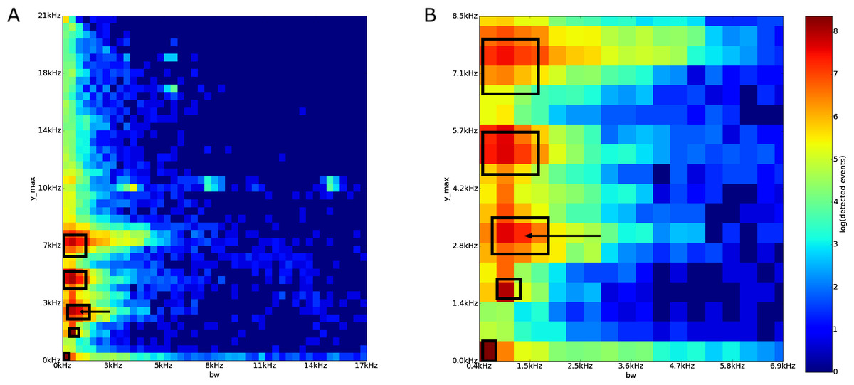
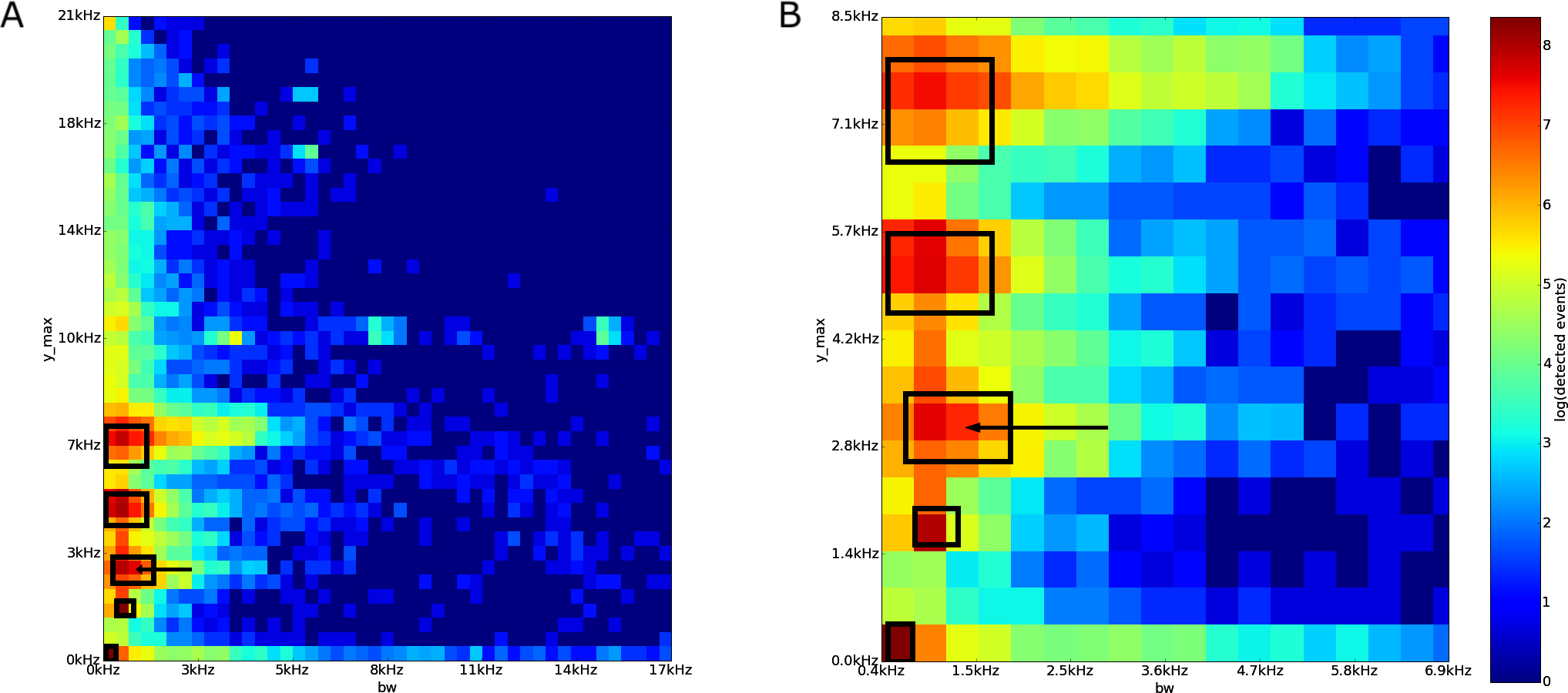
The 50 sampled acoustic events from the area of interest were arranged into six groups (Table 3). The majority of the events (40 out of 50 events) were the second note, “qui,” of the call of the frog Eleutherodactylus coqui. The second largest group is composed of the chirp sound of an Leptodactylus albilabiris (5 events). The third group is two unknown, similar, calls. The fourth group is an event of an Leptodactylus albilabiris chirp with an almost overlapping Eleutherodactylus coqui’s “qui” tone. The last two groups are the call of an unknown insect, and an acoustic event arising from a person speaking on a radio station from an interference picked up by the recorder.
| Type | Count | Percent |
|---|---|---|
| E. coqui’s “qui” | 40 | 80% |
| L. albilabris’ chirp | 5 | 10% |
| Unknown | 2 | 4% |
| L. albilabris’ chirp +E. coqui’s “qui” | 1 | 2% |
| Unknown insect | 1 | 2% |
| Person | 1 | 2% |
Discussion
FLTR algorithm
The FLTR algorithm, in essence, functions as a noise filter for the recording. It takes the spectrogram from a noisy field recording (Fig. 2A), and outputs an image where, in theory, the only variation is due to localized acoustic energy (Fig. 2C). The model imposed on a spectrogram is also very generic in the sense that no particular species or sound is modeled, but rather it models the different sources of acoustic energy. It is reasonable to think that any spectrogram is composed of these three components without a loss of generality: (1) a frequency-based noise level, (2) some diffuse energy jitter, and (3) specific, localized events.
The end product of the flattening step is a spectrogram with no frequency-based components (Fig. 2B). By using the frequency band medians we are able to stay ignorant of the nature of the short-term dynamics in the spectrogram while being able to remove any long-term nuisance effects, such as (constant) background noise or a specific audio sensor’s frequency response. Thus, we end up with a spectrogram that is akin to a flat landscape with two components: (1) a roughness element (i.e., grass leaves) in the landscape and (2) a series of mounds, each corresponding to a given acoustic event. Due to this roughness element, a global threshold at this stage is ineffective. The local trimmed range however is able to enhance the contrast between the flat terrain and the mounds (Fig. 2C), enough to detect the mounds by using a simple global threshold (Fig. 2C). By using a Yen threshold, we maximize the entropy of both the background and foreground classes (Fig. 2D). In the end, the FLTR algorithm has the advantage of not trying to guess the distribution of the acoustic energy within the spectrogram, but rather it exploits robust statistics that work for any distribution to separate these three modeled components.
From the simple intersection test, a sensitivity of 94% assures us that most of the acoustic events in a given recording will be extracted by the FLTR segmentation algorithm, while a positive predictive value of 89% assures us that if something is detected in the recording, it is most likely an acoustic event. Thus, this algorithm can confidently extract acoustic events from a given set of recordings.
From the coverage percentage test, a sensitivity of 85% assures us that most of the acoustic events in a given recording will be extracted by the FLTR segmentation algorithm, while a positive predictive value of 80% assures us that if something is detected in the recording, it is most likely an acoustic event. Thus, this algorithm can confidently extract acoustic events from a given set of recordings.
These performance statistics are obtained from a dataset of only six recordings. Because of this small recording size, biases that may occur due to correlations between acoustic events within a recording cannot be addressed. We tried to reduce this bias by selecting recordings from very different environments. This limitation arises from the fact that manually annotating the acoustic events in a recording is very time consuming. Thus, a limiting factor on the sample size in the validation dataset is that the number of extracted acoustic events for each recording averages to 340 per recording (i.e., for six recordings, we have 2,051 manually labeled acoustic events in total).
The 21 × 21 window parameter was selected in an ad-hoc manner and corresponds to a square neighborhood of a maximum of 10 spectrogram cells around the central cell in the local trimmed range computation step. This allows us to compare each value in the spectrogram to a local neighborhood of about 122 ms and 1.8 kHz in size (assuming a sampling rate of 44,100, or 500 ms and 410 Hz for sampling rate of 10,000 Hz). The α = 5 percentile was also selected ad-hoc. It corresponds to the local trimmed range computing the difference between the 95% and 5% percentiles. This allows the window to contain at least 5% percent of its content as low-valued outliers, and another 5% as high-valued outliers. While these parameter values provided good results, it is not know how optimal they are, nor how the sensitivity and positive predictive value would change if other parameter values were used.
A3 implies that a recording needs to have unsaturated frequency bands (ρ(f) < .5) for the method to work efficiently. This assumption implies that Theorem 1 holds for frequency bands without intense constant chorus (ρ(f) ≤ .5). However, as ρ(f) approaches 1, the frequency band median approaches the median of the aggregate localized energy processes on the frequency band. Thus, at least 50% of the values, more notably the highest values in the aggregate localized energy processes, will always be above b(f). Depending on factors, such as their size and remaining intensity, they could very well be detected. The degradation of the detection algorithm in relation to these assumptions, however, is still to be studied.
FLTR application
In all three sites, the plots with the most joint entropy were cov vs. y˙max, y˙max vs. tod and cov vs. tod. cov measures how well a detection fits within a bounding box and can serve as a measure of the complexity of the event. This value changing across tod and y˙max implies that the complexity of the detected event change across these features. The high joint entropy of y˙max vs. tod is expected, since each variable amounts to being a location estimate: (tod is a location estimate in time while y˙max in frequency) and, thus, subject to the randomness of when (in time) and where (in frequency) an acoustic event occurs. Interestingly, rather than being uniformly distributed, the acoustic events are non-randomly distributed, presumably reflecting the variation in acoustic activity throughout the day. These tod vs. y˙max plots present a temporal soundscape, which provide us with insights into how the acoustic space is partitioned in time and frequency in each ecosystem. For example, in the Sabana Seca and El Verde plots, there is a clear difference in acoustic event density between day time and night time. This correlates with the activity of amphibian vocalizations during the night in these sites (Ríos-López & Villanueva-Rivera, 2013; Villanueva-Rivera, 2014).
An interesting artifact is a downward trending density line that appears on the upper left corner of the plot in y˙max vs. bw in Fig. 5. A least squares fit to this line gives the equation −0.93X + 21.5 kHz, which is close to the maximum frequency of the recordings from El Verde site (these recordings have a sampling rate of 44,100). This artifact seems to arise because the upper boundary of a detected event and bw are constrained to be below this maximum frequency and, for low bw values, y˙max is to be close to the upper boundary of the detected event.
Another useful application of the FLTR methodology is to sample specific regions of activity to determine the source of the sounds. In the sampled area of interest from Sabana Seca, approximately 80% of the sampled of the events were a single note of a call of E. coqui (40 events), and around 10% were the chirp of L. albilabris (5 events). This demonstrates how the methodology can be used to annotate regions of peak activity in a soundscape.
Using the confusion matrix in Table 1 as a ruler, we could estimate that around 94% of the acoustic events were detected and that they conform around 89% of the total amount of detected events.
Conclusion
The FLTR algorithm uses a sound spectrogram model. Using robust statistics, it is able to exploit the spectrogram model without assuming any specific energy distributions. Coupled with the Yen threshold, we are able to extract acoustic events from recordings with high levels of sensitivity and precision.
Using this algorithm, we are able to explore the acoustic environment using acoustic events as base data. This provides us with an excellent vantage point where any feature computed from these acoustic events can be explored, for example the time of day vs. dominant frequency distribution of an acoustic environment (i.e., a temporal soundscape) down to the level of the individual acoustic events composing it. As a tool, the FLTR algorithm, or any improvements thereof, have the potential of shifting the paradigm from using recordings to acoustic events as base data for ecological acoustic research.