
Reconstructing the history of a WD40 beta-propeller tandem repeat using a phylogenetically informed algorithm
- Published
- Accepted
- Received
- Academic Editor
- Claus Wilke
- Subject Areas
- Bioinformatics, Computational Biology
- Keywords
- Ancestor reconstruction, Tandem repeats, Phylogeny, Beta propellers
- Copyright
- © 2015 Lavoie-Mongrain et al.
- Licence
- This is an open access article distributed under the terms of the Creative Commons Attribution License, which permits unrestricted use, distribution, reproduction and adaptation in any medium and for any purpose provided that it is properly attributed. For attribution, the original author(s), title, publication source (PeerJ Computer Science) and either DOI or URL of the article must be cited.
- Cite this article
- 2015. Reconstructing the history of a WD40 beta-propeller tandem repeat using a phylogenetically informed algorithm. PeerJ Computer Science 1:e6 https://doi.org/10.7717/peerj-cs.6
Abstract
Tandem repeat sequences have been found in great numbers in proteins that are conserved in a wide range of living species. In order to reconstruct the evolutionary history of such sequences, it is necessary to develop algorithms and methods that can work with highly divergent motifs. Here we propose a reconstruction algorithm that uses, in parallel, ortholog tandem repeat sequences from n species whose phylogeny is known, allowing it to distinguish mutations that occurred before and after the first speciation. At each step of the reconstruction, both the boundaries and the length of the duplicated segment are recalculated, making the approach suitable for sequences for which the fixed boundary hypothesis may not hold. We use this algorithm to reconstruct a 4-bladed ancestor of the 7-bladed WD40 beta-propeller, using orthologs of the GNB1 human protein in plants, yeasts, nematodes, insects and fishes. The results obtained for the WD40 repeats are very encouraging, as the noise in the duplication reconstruction is significantly reduced.
Introduction
Among the many evolutionary events that shape genes, tandem repeats play a major role as building blocks of protein domains that have structural functions in a cell, and some very useful architectures have been conserved through a wide range of species (Schaper, Gascuel & Anisimova, 2014). One striking example is the 7-bladed beta-propeller of the human GNB1 protein which has orthologs in yeasts and plants: the repetitive nature of this structure is quite obvious in JSmol (Hanson et al., 2013) views such as the one shown in Fig. 1. This repetition is mirrored by the underlying coding sequence that contains nearly 7 repetitions of the WD40 motif, which are short segments of approximately 40 amino acids, featuring a highly conserved W-D dipeptide.
Variation in the number of these building blocks may have an impact on a wide array of geometric parameters such as the diameter of cross-membrane channels, or the area and length of binding surfaces (Andrade, Perez-Iratxeta & Ponting, 2001). For example, the number of W-D repeats in a domain typically ranges from 4 to 16 blades (Li & Roberts, 2001), making up a complex and interesting class of domains whose evolutionary relationships remain unresolved.
The goal of this paper is to propose algorithms and heuristics to reconstruct the evolutionary history of these ancient domains. The main challenges are the lack of sequence similarity between repeats, and the recognition that repeats may not evolve according to a tree-like model—which is a crucial hypothesis in most current approaches.
When form is more important than content, similarity between repeated components can degrade sufficiently to fool computational tools designed to predict them, some of which had to wait for their 3D structural resolution in order to be detected (Kajava, 2012). Reconstructing evolutionary histories of such repeats is particularly difficult, since it relies even more on similarity detection than the prediction problem does.
A second problem in the reconstruction of evolutionary histories is whether the boundaries of the repeated segment remained fixed throughout evolution, or varied from one duplication to the other. The fixed boundaries hypothesis allows for the use of alignments and/or phylogenetic trees that can give global solutions (Gascuel, Bertrand & Elemento, 2005; Sammeth & Stoye, 2006; Tremblay Savard, Bertrand & El-Mabrouk, 2011), but the applications of these techniques are restricted to tandem repeats constrained by biological features, such as the presence of introns separating the repeated segments (Zhuo et al., 2007).
To circumvent these problems, and since ancient domains are likely to have orthologs in several species, we use sets of orthologs to reconstruct, in parallel, their common evolutionary history. The backbone of the method (Benson & Dong, 1999) is the only known algorithm that does not rely on the fixed boundary hypothesis (Rivals, 2004). The Benson and Dong algorithm is parsimony-based, and we extend it using the same principle, given the computationally intensive nature of our approach.
We illustrate our approach using a set of six GNB1 ortholog W-D domains in mammals, plants, yeasts, nematodes, insects and fishes: these were shown to share their evolutionary history in at least two independent studies (Chaudhuri, Soding & Lupas, 2008; Schaper, Gascuel & Anisimova, 2014). We give evidence that the fixed boundary hypothesis might not apply, and we reconstruct a 4-bladed ancestor of the 7-bladed W-D GNB1 beta-propeller that matches living fossils such as slime molds.
Methods
Preliminaries
A tandem repeat is a sequence composed of the repetition of approximate copies of a motif, where the first or the last repetition may be truncated. For example, the tandem repeat:
CC GTTAC GTTACC GTAGCcontains approximate repetitions, separated by spaces, of the motif GTTACC.
When the motif and the copies have the same length, we call this length a period. With insertions and deletions in the copies, it is always possible to transform a tandem repeat such that all the complete copies have the same length. For example, the above sequence can be rewritten, by inserting two gaps, as: CC GTTA-C GTTACC GT-AGC. Once all copies have the same length, the trivial multiple alignment of the successive copies is called a self-alignment.
The problem of self-aligning a tandem repeat sequence while optimizing any interesting score—sum-of-pairwise-distances, star and tree alignments, etc.—is NP-hard (Elias, 2006), and is at the heart of every reconstruction strategy (Rivals, 2004). However, in the case of tandem repeats that code for protein domains whose structure is resolved, such as in Fig. 1, structure-guided alignments can be used to infer the corresponding self-alignments (Chaudhuri, Soding & Lupas, 2008).
The history of a tandem repeat is a description of how it went from one copy of the motif in the ancestor to the many copies in the observed sequence. This can be formalized using various models of evolution. All these models include mutations, insertions and deletions of nucleotides that affect a single copy of the motif, and duplications that replace a segment of k copies of the motif by two consecutive segments both identical to the initial segment (Benson & Dong, 1999). More elaborate models will consider operations that transform a segment into two or more identical segments (Gascuel, Bertrand & Elemento, 2005), deletion of copies (Sammeth & Stoye, 2006), or even inversions and speciations (Tremblay Savard, Bertrand & El-Mabrouk, 2011). The main hurdle in the reconstruction problem is the fact that more than a billion years of evolution can significantly blur the similarity of the sequences, thus rendering quantitative comparison tools meaningless.
Algorithmic approaches vary according to the evolutionary model, and more fundamentally according to assumptions on the behavior of duplications, linked to the concept of parsing. Given a period p, a parsing of a tandem repeat is the determination of the boundaries of the copies of a repeated motif of length p (Matroud et al., 2012). For example, here are two different parsings of the example sequence:
CC | GTAA-C | GTTACC | GT-AGC
CCGTA | A-CGTT | ACCGT- | ACCIn the fixed boundaries model, the boundaries of all duplications are boundaries of the same parsing; in the dynamic boundaries model, parsing may vary from one duplication to the next. With the fixed boundaries hypothesis the reconstruction problem can be reformulated as the construction of a duplication tree, opening up the vast repertoire of phylogenetic tools. In contrast, the more general dynamic boundaries hypothesis implies that exhaustive searches must be repeated at each step (Benson & Dong, 1999), and the evolutionary history cannot be represented by a tree (Jaitly et al., 2002).
Architecture of the GNB1 beta-propeller
The guanine nucleotide-binding protein (GNB1) is a protein characterized by a tandem repeat of seven copies of the WD40 protein motif (PFAM00400). These fold in a three-dimensional cylindrical structure, whose top view, as seen in Fig. 1, looks like a propeller with seven blades. Each blade is a beta sheet consisting of four strands, denoted A, B, C, and D, from the centre of the propeller to its circumference. However, the strands appear in the tandem repeat in the following order:
D1A2B2C2D2A3B3C3D3A4B4C4D4A5B5C5D5A6B6C6D6A7B7C7D7A1B1C1Thus, there are at least two competing parsings of the tandem repeat: one that preserves the integrity of the 3D blades, with motif ABCD, and one that maximizes the number of complete copies, with motif DABC. In view of this particularity, we reject the fixed boundaries hypotheses in favor of dynamic boundaries, leaving open the possibility of eventually detecting fixed boundaries.
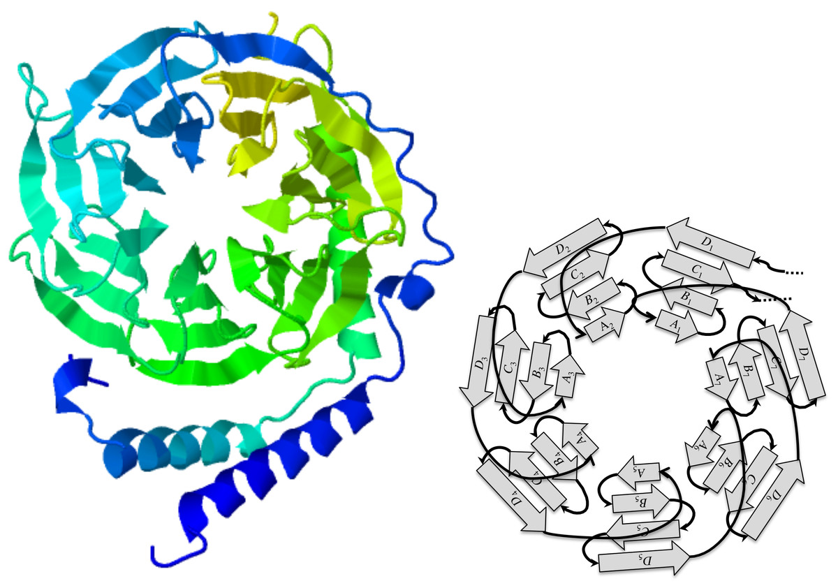
Figure 1: The GNB1 beta-propeller.
In this JSmol (Hanson et al., 2013) ribbon diagram view of a GNB1 beta-propeller ortholog (PDB:1TBG; GenPept:P62871), the blades are displayed as seven triangles organized in a circle, like a propeller. Each blade is composed of four strands, labeled A, B, C, and D starting from the inner one. Reading the protein sequence from N-terminus to C-terminus, the first strand is the D strand of the upper right blade (D1), followed by the A, B, C strands of the upper left blade. The A, B, C strands of the upper right blade (A1, B1 and C1) are the last strands of the protein sequence. This implies that, sequence-wise, blades are shifted with respect to the corresponding 3D units.
The WD40 protein motif, which actually codes for the components of a blade, is quite common (Stirnimann et al., 2010), and is responsible for a variety of propellers ranging from 4 to 8 blades, whose ancestry can be traced back to both recent rounds of duplications, and very ancient ones (Chaudhuri, Soding & Lupas, 2008). The GNB1 propeller falls in the latter category, and has been found in all sequenced eukaryotes species.
A GNB1 ortholog tandem repeats dataset
We selected a set of GNB1 orthologs using the Ensembl (Flicek, Amode & Barrell, 2014) database, and BLAST (Altschul et al., 1990) in the case of Arabidopsis. Table 1 gives the accession numbers and the positions of the WD40 tandem repeat in each sequence. Figure 2 shows the current consensus of the phylogeny of the six species (Dunn et al., 2008).
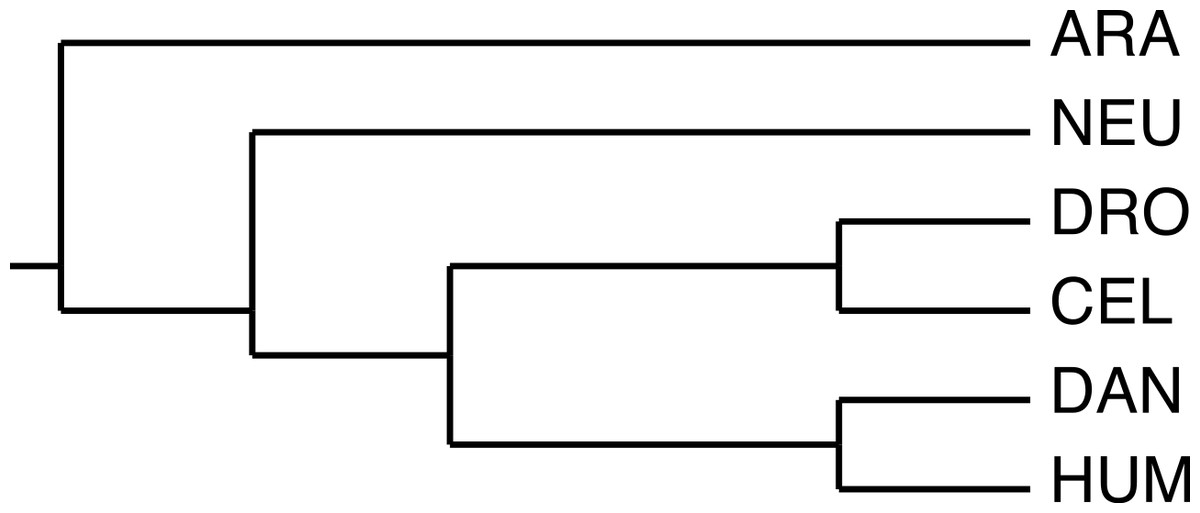
Figure 2: The phylogeny used by the algorithm.
The species phylogeny from Dunn et al. (2008) used as input in the reconstruction algorithm.
We used the structure-guided alignment of GNB1 given in Chaudhuri, Soding & Lupas (2008) to identify insertions and deletions of the human sequence within the WD40 motif. We then aligned the human sequence with A. thaliana and N. crassa sequences in order to transfer the insertions and deletions from the human, and to identify further deletions in A. thaliana and N. crassa. The alignment is shown in Fig. 3. The three remaining species inherited the same insertions and deletions as the human.
The resulting amino acid sequences have all the same length. These sequences are ortholog tandem repeats with 6.8 copies of the WD40 motif, as shown in the self alignment of the human sequence in Fig. 4. The underlying genomic sequences have a length of 864 bp; in the rest of this paper, they will be denoted by the names HUM, DAN, DRO, CEL, NEU, ARA, as in Table 1.
For comparison purposes, we computed the initial alignment with the standard tools Clustal Omega (Sievers et al., 2011) and Muscle (Edgar, 2004). Of the eleven or so mutations proposed by Chaudhuri et al., Clustal finds 7 of them, and Muscle only 2, we thus used the Clustal alignment. No classical aligner can predict, as Chaudhuri et al. do with structural knowledge, the two deletions that occur in all sequences. These deletions are necessary information for the computation of self-alignments.
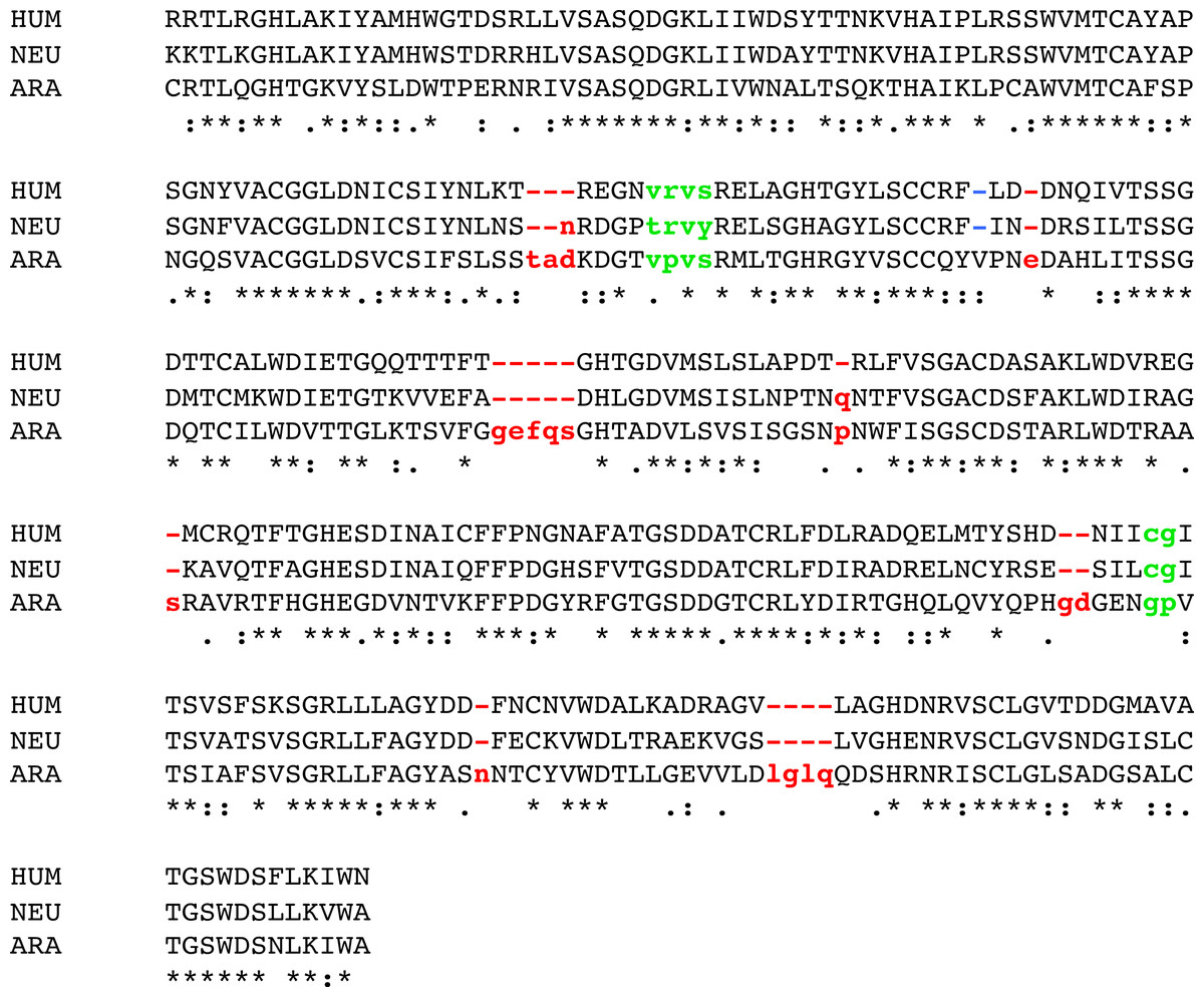
Figure 3: Alignment of three GNB1 ortholog sequences.
The beta-propeller domain of the three GNB1 ortholog sequences from HUM, NEU and ARA were aligned using Clustal Omega (Sievers et al., 2011). The alignment was edited as shown: two blocks (green) were removed from all the sequences, according to the structural alignment of Chaudhuri, Soding & Lupas (2008) that suggested that these blocks do not belong to the structure; one gap (blue) was inserted in the HUM and NEU sequence, again according to Chaudhuri, Soding & Lupas (2008); eight blocks (red) were removed from the NEU and ARA sequences corresponding to gaps in the HUM sequence. The remaining sequences, DAN, DRO and CEL, have exactly the same editions as the HUM sequence, since they align without gaps. The six resulting edited sequences have all the same length, 288 aa. The nucleotide sequences coding for these sequences were then extracted, to yield the main dataset of six sequences of length 864 bp.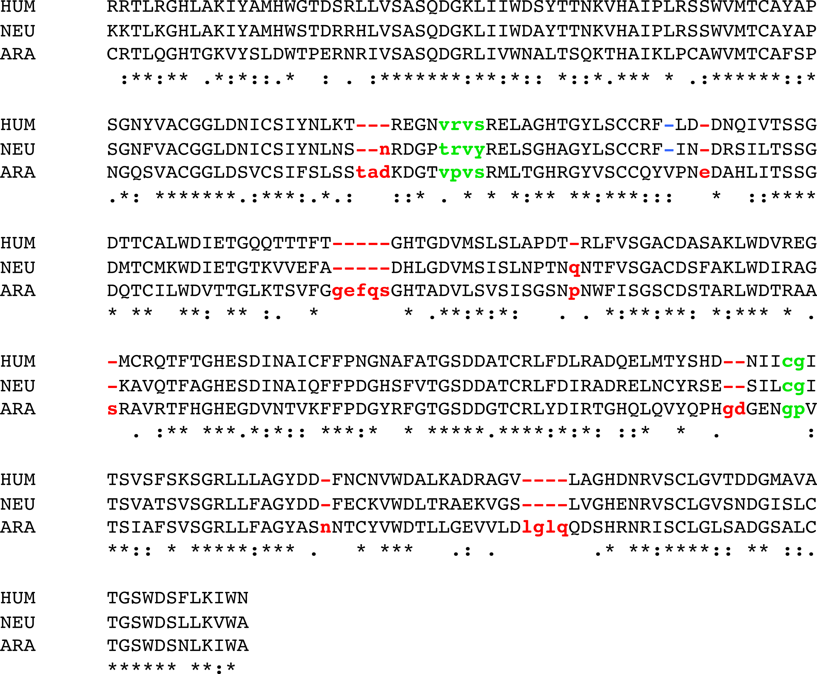
Figure 4: Self-alignment of the human sequence.
A self-alignment of HUM sequence shows a 42 amino acids long tandem repeat of 6.8 copies of the WD40 domain.The highlights of the WD40 repeat (Stirnimann et al., 2010) are illustrated by the high conservation of the G-H and W-D groups (in blue), and the conserved D residue (in red).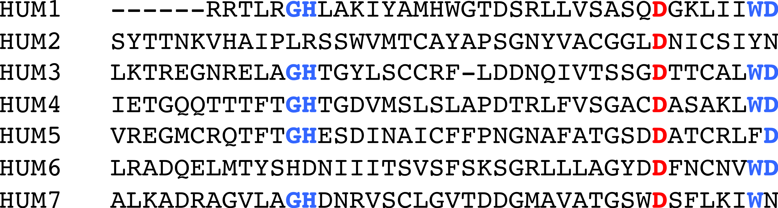
Pinpointing the most recent duplication
Here we describe how to detect the most recent duplication in a tandem repeat, first by using species separately, then by processing the six species in parallel. The first model follows closely the Benson & Dong model (1999). The second is an enhanced model that uses phylogenetic trees of ortholog domains to distinguish mutations that occurred before all speciation events, from mutations that occurred after speciation.
Using a single species
After a duplication of a segment, the two copies are identical. If each copy accumulates mutations independently and uniformly, which is equivalent to a molecular clock hypothesis among the repeated segments, the most recent duplication should be indicated by the pair of segments that have the least differences. This leads to the following definition of a cost function, whose value is proportional to the number of mutations that separates two segments, and called the contraction cost (Benson & Dong, 1999). Let S be a nucleotide sequence, ℓ be a period length, and the edit distance given by δ(n1, n2) = 0 if nucleotides n1 and n2 are equal, otherwise δ(n1, n2) = 1. We define the contraction cost of two consecutive segments of length ℓ at position pos of the sequence S as: (1) The normalization of the cost will allow the comparison of costs between different values of ℓ.
Given a motif of length p and a tandem repeat sequence S, the position of the most recent duplication of one or more copies of the motif should be a position in S that minimizes C(pos, ℓ), for all values of pos and ℓ ∈ {k∗p | k ≥ 1} for which C(pos, ℓ) is defined.
For the three GNB1 ortholog sequences HUM, NEU and ARA, we tested all possible periods and obtained minimal values for p = 126. Figure 5 shows the values of C(pos, 126) for each species. The prediction that no meaningful minimal values would emerge is confirmed both by the random nature of the HUM curve, and by the fact that, although these three sequences share the same duplication history, they do not agree on its most recent development.
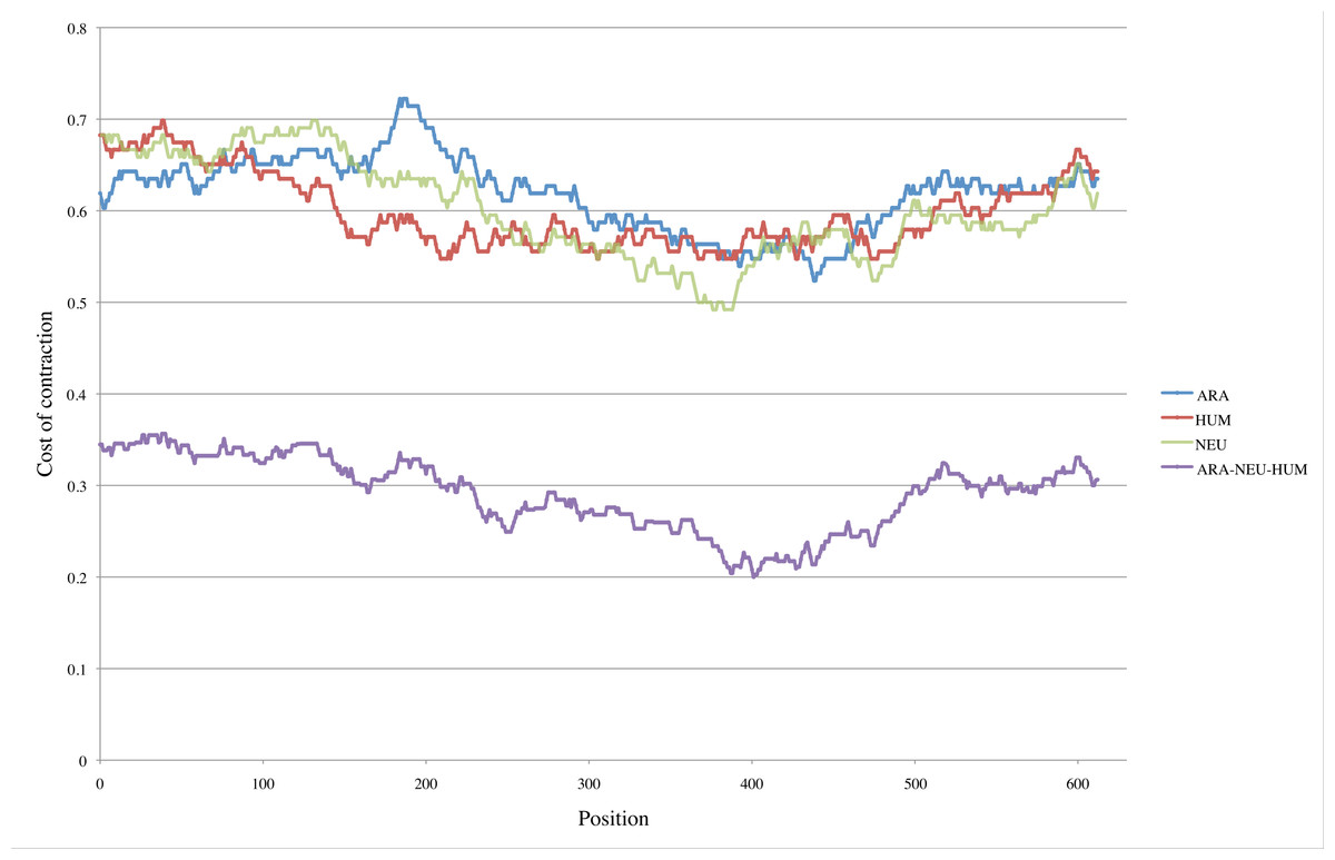
Figure 5: Pinpointing the most recent duplication.
Top three curves: For each position pos in the three nucleotide sequences HUM, NEU and ARA, we computed the cost C(pos, 126) of contracting segments [pos..pos + 125] and [pos + 126..pos + 251]. The positions where minimal values are attained presumably indicate where the most recent duplication occurred. For the HUM sequence (red curve), positions corresponding to minimal values are scattered within the interval [209..477]. Although the intervals are smaller in the case of NEU and ARA (green and blue curves) those intervals do not even intersect. Bottom curve: This is the curve obtained by combining the data from HUM, NEU and ARA. The values of all costs are drastically reduced, with the absolute minimum reduced by more than half (0.492 for the NEU curve compared to 0.200 for the combined curve). The interval of positions where minimal values are attained is reduced to [387..403].
Using multiple species
In this section, we use the same global approach as the preceding section, but we estimate the cost of a contraction based on the reconstruction of the ancestral tandem repeat of n extant tandem repeats who share the same duplication history, and whose phylogeny is known. We replace the distance δ(n1, n2) between nucleotides—whose value is 0 or 1—by a cost that ranges in the interval [0..1]. The following small example illustrates the method.
Consider the following three ortholog sequences, each with a tandem repeat of two repetitions of a motif of length 3.
     1  2  3     1′ 2′ 3′
Sp1  T  A  G  |  T  T  T
Sp2  C  A  A  |  A  T  T
Sp3  T  C  C  |  A  T  T
At positions 1 and 1′, both species Sp2 and Sp3 have a mutation compared to Sp1. If the phylogeny is (Sp1, (Sp2, Sp3)), then all parsimonious reconstructions of the ancestral nucleotide give T for both positions 1 and 1′ as in Tree 1 of Fig. 6. In the case of positions 2 and 2′, all parsimonious reconstructions, such as Trees 2a and 2b of Fig. 6, give A for position 2, and T for position 2′.
For positions 3 and 3′, some reconstructions have a mutation that precedes speciation and some do not. Figure 6 gives four possible reconstructions: Trees 3a, 3b and 3c have one mutation before speciation and Tree 3d does not.
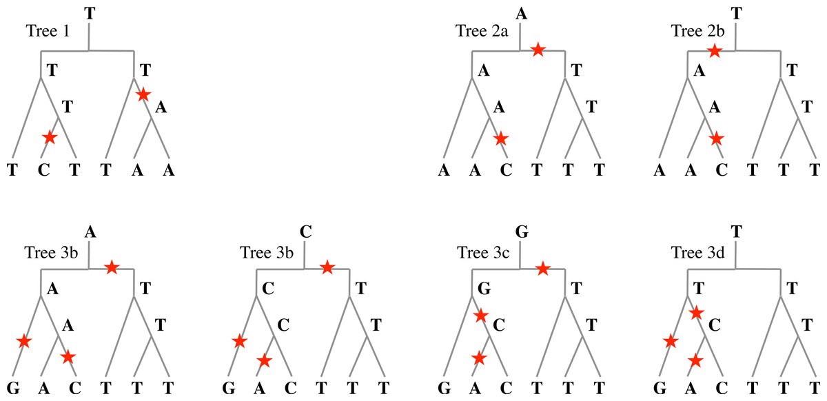
Figure 6: Evolutionary histories.
Examples of evolutionary histories of a nucleotide that underwent one duplication followed by two speciation events. In Tree 1, two mutations occurred after speciation: any parsimonious reconstruction from extant nucleotides would agree with this. In Trees 2a and 2b, one mutation occurred before any speciation, and one after: again, any parsimonious reconstruction would agree; however, the ancestral nucleotide could be A or T. In Trees 3a to 3d, four parsimonious reconstructions with three mutations are given. The number of mutations before speciation can be 0 or 1, and the ancestral nucleotide can be A, C, G, or T.
Formally, given n ortholog tandem repeats, from n species whose phylogeny is given by tree , construct the tree whose root is a duplication node, with two copies of tree labeling its two children. The leaves of the left subtree are labeled by the nucleotides at position pos for each species, and the leaves of the right subtree are labeled by the nucleotides at position pos + ℓ.
Consider the set of all labelings of all nodes of tree such that the total number of mutations on the edges is minimal. Let m(pos) be the number of labelings in with one mutation between the root and one of its children. Then the contraction cost for position pos is defined by: . Note that, in a parsimonious labeling, there is at most one mutation between the root and its children.
The contraction cost of two consecutive segments of length ℓ at position pos of the sequence S is defined by: (2)
We tested this new cost function with the three ortholog tandem repeats ARA, HUM and NEU, in parallel, to obtain the bottom curve of Fig. 5: the positions where the minimal, or near minimal costs are attained are in a small interval, and the contraction costs are nearly halved with respect to the former cost function.
Since the contraction cost for a position, , is a number between 0 and 1, the total number of mutations as computed by C(pos, ℓ)∗ℓ is not necessarily an integer. When we want to evaluate the number of mutations necessary to perform a contraction, we use the formula:
Contractions and iterations
The labels at the root of different labelings in are the putative ancestors of the nucleotides at position pos and pos + ℓ, this set of ancestors is denoted by A(pos).
To perform the contraction of two segments of length ℓ on a tandem repeat at position pos, we replace the two segments by a single segment. This segment is the sequence of sets A(i) for pos ≤ i < pos + ℓ. For example, the contraction of the tandem repeat in the three sequences TAGTTT, CAAATT, and TCCATT used in Fig. 6 would be:
{T}{A,T}{A,C,G,T}After a contraction is performed, it is possible to iterate the procedure by choosing the next more recent duplication. In this case, the leaves of the tree will be labeled by sets of nucleotides instead of single nucleotides.
Clearly, when using multiple species, iterated contractions may be performed only on ancient duplications, that is those which preceded speciation. In the case of GNB1 orthologs, strong evidence supports the fact that all duplications of the WD40 motif preceded all speciations, at least up to the common ancestor of plants and animals. A compelling example of this was shown by Schaper and colleagues in the recent large scale study (Schaper, Gascuel & Anisimova, 2014). All approaches are based on the same principle that, when analyzed by phylogenetic tools, the motifs regroup by their position in the tandem sequence rather than by the species they belong to. We provide, in Fig. 7, yet another evidence of this.
Figure 7: Evidence of duplications followed by speciations.
In order to establish the fact that all duplications of the GNB1 beta-propeller preceded the speciation events, we parsed the HUM, NEU and ARA nucleotide sequences in seven ‘blades’, numbered as in Fig. 4. A phylogenetic tree was then constructed using Dnapars (Felsenstein, 1993), showing that the tree supports the fact that duplication events preceded speciation events. Different parsing choices and phylogenetic tools all yielded trees in which the blades grouped by their number rather than by species (data not shown).
The contraction procedure may be iterated as often as the sequence is long enough to be contracted. However, it is clear that in some circumstances further contractions are not recommended, as the experiment with the HUM sequence showed in Fig. 5. Before performing a contraction, one should make sure that the interval of positions with minimal costs is small, and that these costs are well below the random costs of performing a contraction anywhere else. The next section contains some further examples of these situations.
Algorithms and complexity
The complete procedure is composed of the following steps, taking as input a motif of known length p and a set of n ortholog tandem repeats of the motif:
-
Create a dataset of n tandem repeats of the same length, using insertions and deletions within copies of the motif. If a structure-guided alignment exists, use it.
-
Find the values of (pos, k∗p), k ≥ 1 that minimize, or nearly minimize, the contraction cost C(pos, ℓ), as defined by Eq. (1) or Eq. (2).
-
Decide whether there is sufficient evidence to confirm the position of a further contraction. If not, stop.
-
Perform the contraction, and go to Step 2.
Only Steps 2 and 4 can be solved by algorithms, and, fortunately, efficient algorithms are available for these tasks. The computation of contraction costs as defined by Eq. (1) is rather trivial. The computation of C(pos, ℓ) as defined by Eq. (2), which calls for the enumeration of all parsimonious labeling of a tree is more complex. Fortunately, there exists an algorithm developed by Sankoff (1975) whose data structure can be used to compute both and the set of A(pos) of possible ancestors.
Define the cost of a labeling of a tree to be the number of edges that have different labels at their extremities. At each vertex v of the tree , we compute, for each symbol b in {A, C, T, G, - }, the minimal cost M(v, b) of a labeling of the subtree rooted at v, with base b labeling vertex v; and the number N(v, b) of such minimal cost labelings. A classical dynamic programming algorithm (Sankoff, 1975) is used to fill out the structure. The values of these parameters at the root R of , and at its left and right children LR and RR, are sufficient to compute A(pos) and the contraction cost at position pos. namely:
-
A(pos) is the set of bases b for which M(R, b) is minimal.
-
.
-
.
These are all polynomial algorithms, but the extensive computations involved in making tens of thousand of experiments prompted us to implement these with various speed-up techniques (Lavoie-Mongrain, 2014).
Experimental set-up
We ran 30 × 30 × 30 = 27,000 experiments computing the total cost of the first four contractions yielding the 27,000 data vectors (p1, p2, p3, p4) and (c1, c2, c3, c4), where ci is the contraction cost at position pi. The positions p1 span the 30 lowest costs of a first contraction; for each value of p1, the positions p2 span the 30 lowest costs given a first contraction at p1; for each pair (p1, p2), the positions p3 span the 30 lowest costs given contractions at p1 and then p2. Position p4 is the smallest position, for a fourth contraction, with lowest cost. The 72 best results for the first three contractions are available in Table S1. The computation time for the 27,000 experiments was around 21/2 hours (148.5 min) on a 3 GHz processor with 8 GB RAM.
Although we tried contractions of length k × 126, with k > 1, none of them made it in the 30 lowest costs at any iteration.
Results
Using the six ortholog tandem repeats HUM, DAN, DRO, CEL, NEU and ARA, with the phylogeny of Fig. 2, we ran 27,000 experiments minimizing the total cost of going from seven blades to three blades. All scenarios predict four contractions of length 126. This set of experiments allowed us to study the behavior after one, two, three or four contractions.
The 18 optimal scenarios predicted a total of 122 mutations to perform the four contractions, and 296 near optimal scenarios predicted a total of 123 mutations. Table 3 sums up the principal characteristics of these 314 scenarios giving, for each contraction, the interval of positions in which minimal or near minimal values were obtained, its width, and the range of its costs.
| Contraction | Interval | Width | Costs |
|---|---|---|---|
| 1 | [383..437] | 55 | 0.209–0.219 |
| 2 | [237..305] | 69 | 0.198–0.235 |
| 3 | [312..333] | 22 | 0.229–0.267 |
| 4 | [58..164] | 107 | 0.270–0.306 |
Since the cost of the fourth contraction is in the upper range of cost values (an example using one of the optimal scenarios is shown in Fig. 8), and is predicted at positions ranging from 58 to 164, which is a very wide interval given that the period is 126, we halted the reconstruction process before the fourth contraction, leading us to concentrate on scenarios with three contractions yielding a 4-bladed ancestor.
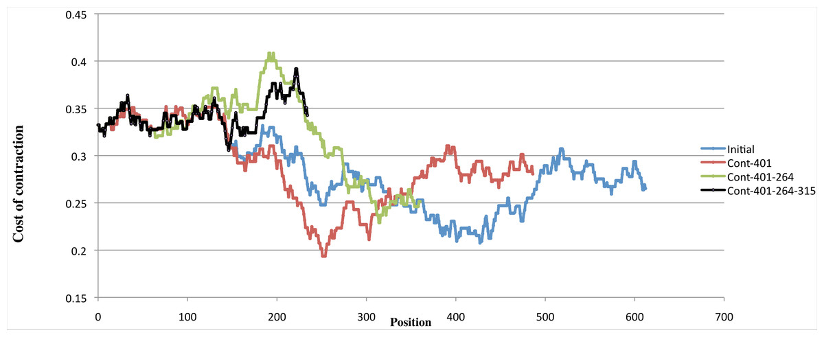
Figure 8: Variation of costs over four contractions.
Example of the variation of the cost of four contractions using one scenario with minimal cost. The blue curve shows, for each position of the input sequence, the cost of performing a contraction of length 126 at that position. The red curve shows the contraction costs computed on the sequence obtained by contracting the input sequence at position 401. The green curve shows the contraction costs computed on the sequence obtained by contracting the input sequence at position 401 then at position 264. The black curve shows the contraction costs computed on the sequence obtained by contracting the input sequence at position 401, at position 264, and then at position 315. While the first three curves have well defined minima, the fourth curve is in the upper range of all curves, showing that performing a fourth contraction might be meaningless.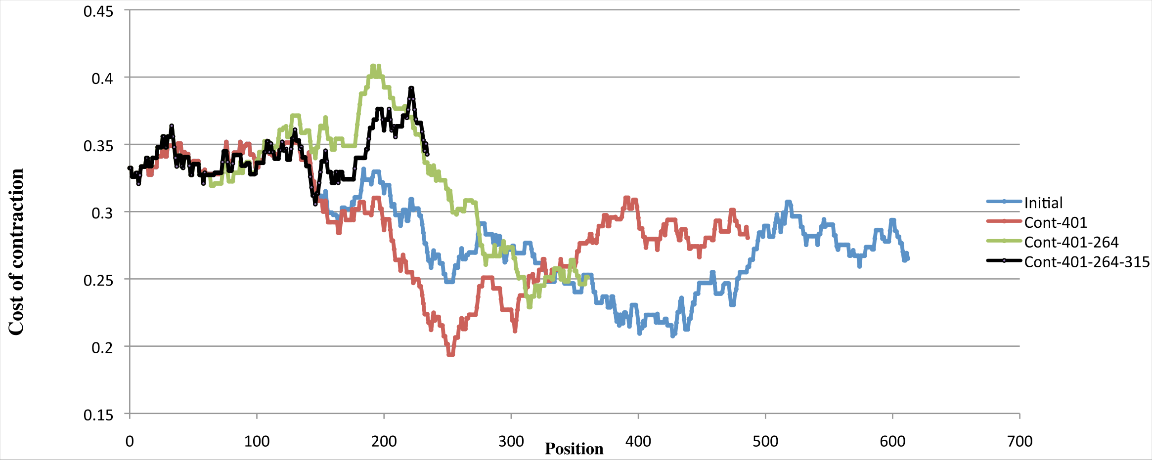
The 4-bladed ancestor
Of the 27,000 experiments, 6 optimal scenarios predicted a total of 83 mutations to perform three contractions, and 66 near optimal scenarios predicted a total of 84 mutations. Table 3 shows the same statistics as Table 2 for these 72 scenarios. The complete results for these experiments are in Table S1.
| Contraction | Interval | Width | Costs |
|---|---|---|---|
| 1 | [383..402] | 20 | 0.209–0.218 |
| 2 | [251..264] | 14 | 0.188–0.221 |
| 3 | [312..322] | 11 | 0.228–0.253 |
We analyzed all 72 reconstructions of the 4-bladed ancestor corresponding to the 72 best results. These reconstructions are remarkably similar, which is not completely surprising given the narrow ranges of possible first, second and third contraction, as can be seen in Table 3, and Fig. S1.
For each triplet of positions, we performed the three contractions, and then translated the contracted part using the extended one-letter amino acid code (Cornish-Bowden, 1985) that assigns the letter B to the sets of amino acids {D, N}, and the letter Z to the set {E, Q}, see Fig. 9.
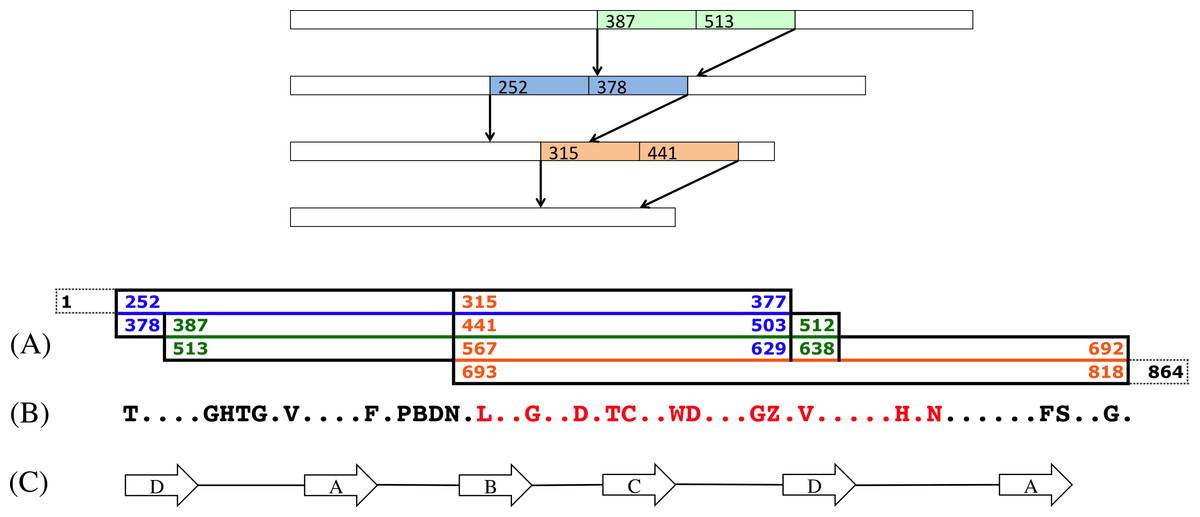
Figure 9: A scenario of three contractions.
Top: A scenario of three contractions at positions 387, 252 and 315. (A) This diagram shows the positions of the original sequence that have been contracted. The first one, in green, is the contraction of the intervals [387..512] and [513..638]. The second one, in blue and overlapping the green contraction, is the contraction of intervals [252..377] and [378..503]. The last contraction, in orange and overlapping the two other contractions, starts at position 315, and runs up to the original position 818, leaving 46 non contracted nucleotides, in dashed lines, at the end of the sequences. (B) This is the reconstructed amino acids sequence of the contracted segment. Amino acids B and Z stand, respectively, for the sets of amino acids {D, N} and {E, Q} (Cornish-Bowden, 1985). The amino acids in red correspond to the pattern that was found in the Slime mold GNB1 protein (see text). (C) The positions of the strands A, B, C and D in the contracted sequence.
All reconstructions left undisturbed both the first two repeats—positions 1–251—and the last 39 positions (see Fig. S1). All reconstructions agreed on the following translated middle part sequence (see Fig. S2), where dots indicate unresolved amino acids:
GHTG.V....F.PBD.....G..D.TC..WD...GZ.V.....H.N......FS..Gand 69 sequences (96%) agreed with the pattern:
GHTG.V....F.PBD..L..G..D.TC..WD...GZ.V.....H.N......FS..GSearching these patterns in various protein databases yields no result. However, searching for the longest (sub)pattern that has at least one hit, gives very interesting results. This pattern is:
L..G..D.TC..WD...GZ.V.....H.NThe pattern was not found in the six sequences that were chosen for the current experiment. However, there were 32 hits in the TrEMBL protein database (Bairoch & Apweiler, 2000) using ScanProsite (de Castro et al., 2006). Of these hits, two were for the slime molds Dictyostelium discoideum and Dictyostelium purpureum, whose divergence is presumed to date back to 400 million years (Parikh et al., 2010). The rest of the hits are all Basidiomycota, which is a fungus phylum: these hits include mostly rots and smuts, with some yeasts, and two edible mushrooms, the Shitake and the Champignon de Paris.
Discussion and Conclusions
While phylogenetic tools and data have been used for tandem repeat reconstruction, it was always in the context of the fixed boundaries hypothesis. The procedure that we presented in this paper constitutes, to the best of our knowledge, the first attempt to systematically use phylogenetic data to reconstruct the evolutionary history of tandem repeats with dynamic boundaries. The choice of parsimony was based on two considerations. First, we are generalizing a parsimony-based algorithm, and, second, since we are using a very computationally intensive algorithm, efficiency is an issue: computation of the cost functions is at the core of the algorithm, it has to be simple. In the future, it would be interesting to define more sophisticated cost functions since we now know the value of basic parameters, such as the period.
In a recent paper (Schaper, Gascuel & Anisimova, 2014), the authors found 3,091 tandem repeats in human proteins, of these, 17% are conserved since the root of the vertebrates. This means that there are potentially 525 sequences that could be studied by techniques presented in this paper. The phylogenetic methods proposed in that paper, based on a fixed boundary tandem repeats, are much more efficient than our exhaustive search approach and should be used whenever the fixed boundary hypothesis is suspected to apply, such as when the repeated units are bound by exons (Schaper, Gascuel & Anisimova, 2014). However, as the example of WD40 beta-propeller tandem repeat suggests, duplication histories with dynamic boundaries should not be readily excluded.
Are the proposed 4-bladed ancestor, or the common motif that we identified, realistic? It is hard to answer yes or no, but a few good arguments plead in favor of this ancestor. Taking an a posteriori look back at Fig. 5, in which we studied the species separately, one can see that the NEU sequence is a very good predictor for the consensus position of the most recent duplication. It is also the most simple species in our dataset, and the common motif that we found points to early branching or slow evolving organisms, such as slime molds.
Given the fact that the first repeat interacts with the last one in order to close the circular structure of the beta-propeller, as seen in Fig. 1, it seems very plausible that the expansion of the number of blades in propellers should leave the beginning and end of the sequence undisturbed, since they probably need co-evolution to properly glue the structure. This may explain why we could not reliably predict any contraction overlapping the first two repeats, or the last 12 residues.
Most importantly, no overwhelming evidence supports the hypothesis of fixed boundaries in the WD40 beta-propeller tandem repeat. As Fig. 9C shows, while the boundaries of the second most recent duplication coincide with the boundaries of a DABC parsing of the WD40 motif, the boundaries of the most recent are a little bit offset from those of the DABC parsing, and the boundaries of the third most recent do not agree at all with those of the DABC parsing. This pattern is true for all the 72 best results.