Enhancing micro-architecture optimization using explainable fuzzy neural networks with multi-fidelity reinforcement learning
- Published
- Accepted
- Received
- Academic Editor
- Arun Somani
- Subject Areas
- Algorithms and Analysis of Algorithms, Artificial Intelligence, Computer Architecture, Optimization Theory and Computation, Neural Networks
- Keywords
- Fuzzy, Microarchitecture, Approach, Optimization, Human, Explore
- Copyright
- © 2026 Alkhiri et al.
- Licence
- This is an open access article distributed under the terms of the Creative Commons Attribution License, which permits unrestricted use, distribution, reproduction and adaptation in any medium and for any purpose provided that it is properly attributed. For attribution, the original author(s), title, publication source (PeerJ Computer Science) and either DOI or URL of the article must be cited.
- Cite this article
- 2026. Enhancing micro-architecture optimization using explainable fuzzy neural networks with multi-fidelity reinforcement learning. PeerJ Computer Science 12:e3429 https://doi.org/10.7717/peerj-cs.3429
Abstract
Micro-architecture design space exploration (DSE) is essential for the optimization of processor performance. However, existing approaches generally fall short in interpretability, preventing designers from comprehending and fine-tuning decisions. In this article, we develop an Explainable Fuzzy Neural Network (FNN) framework coupled with multi-fidelity Reinforcement Learning (RL) for micro-architecture optimization. Instead, this proposed approach is a fuzzy-based one. It induces readable design rules by mimicking a neural network without limiting its flexibility. We employ a multi-fidelity RL strategy to simultaneously enable fast evaluation on analytical models, as well as perform accurate design validation on register transfer level (RTL) simulations to save time and guarantee correctness. Opportune learning of this kind greatly lowers computation costs and retains solutions of suitable quality. The FNN learns interpretable decision rules in an unsupervised fashion, allowing the designer to visualize optimization paths taken and incorporate domain knowledge to guide exploration. Our experiments show that our approach substantially improves the efficiency and accuracy over state-of-the-art DSE methods, yielding near-optimal micro-architectures with a very small sample budget. The interpretability of the framework also enables designers to visually inspect and optimize architectural trade-offs. Nearly closes the gap between black-box optimization and human-guided decision-making, our methodology establishes a solid groundwork for both explainable and efficient micro-architecture DSE, offering a pathway for future work that turns to more transparent and modelled methods of processor design.
Introduction
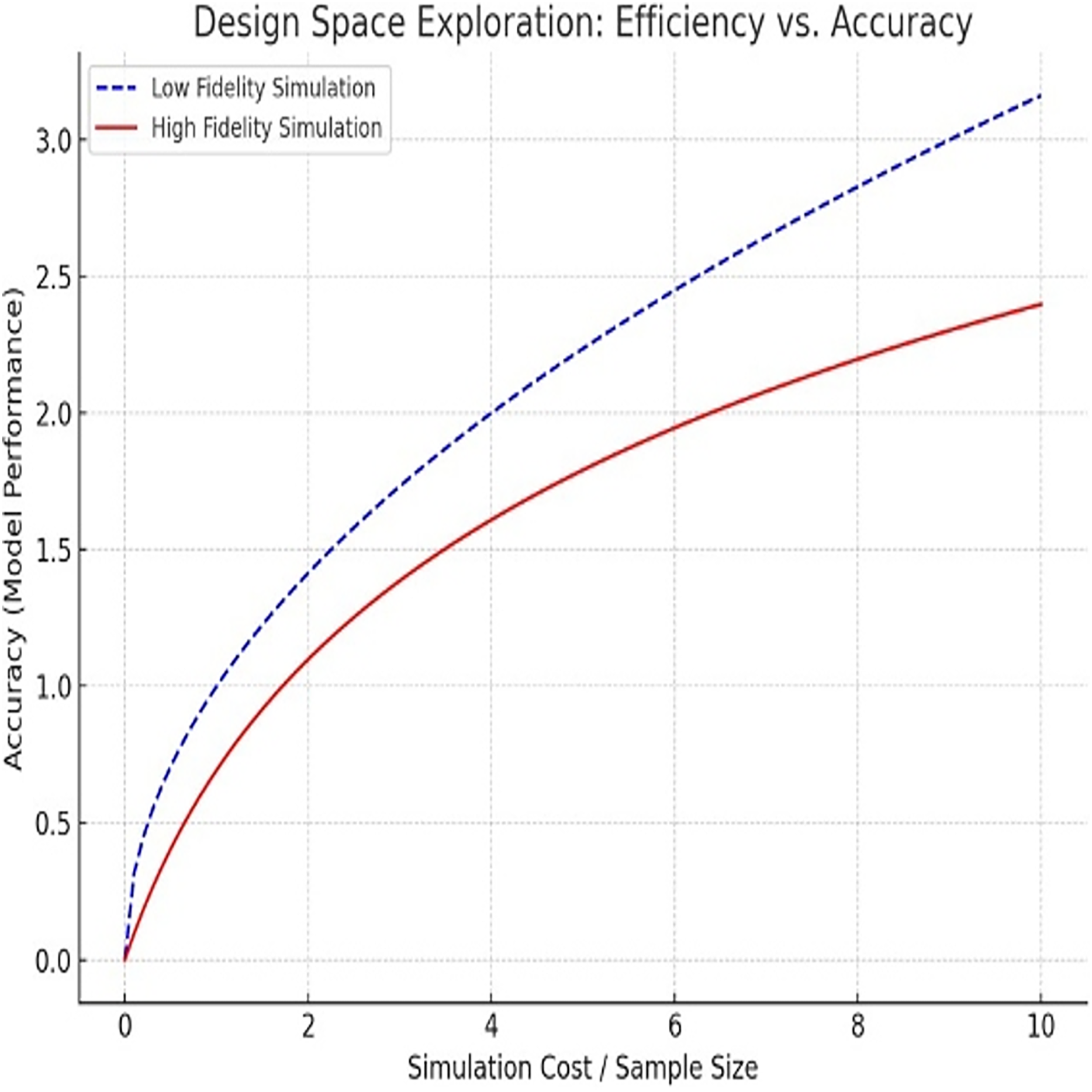
Micro-architecture design space exploration (DSE) plays a crucial role in optimizing processor performance. DSE evaluates a wide range of potential processor architectures, but verifying multiple configurations is challenging due to the sophistication of contemporary processors. Traditional approaches are not able to process the exponentially increasing space of design (Fig. 1). Thus, the practicalities of existing approaches should strike a balance between the efficacy with which they assess evaluations and effective efficiency (Fan et al., 2024).
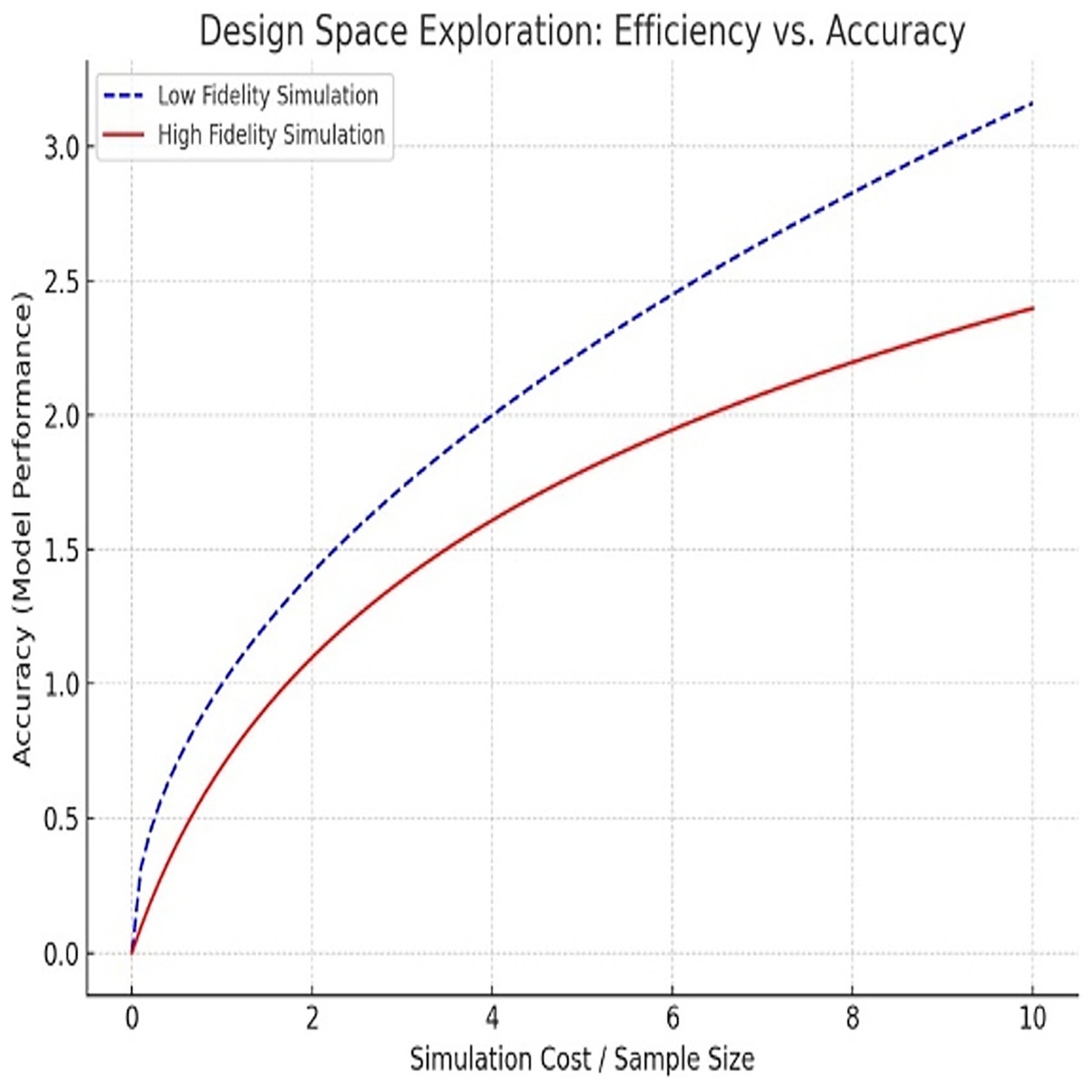
Figure 1: Design exploration between efficiency and accuracy.
Existing automated DSE approaches are often black-box models, lacking transparency and making decisions hard for designers to interpret. With these black-box techniques, designers have difficulties in utilizing their expertise. This lack of transparency is undesirable since slight design manipulations have had a huge impact of performance, power, and cost.
This article presents a new DSE-based approach based on Explainable Fuzzy Neural Networks (FNN) and Multi-Fidelity Reinforcement Learning (MFRL). The methodology will allow interpretability and efficiency. Fuzzy logic produces intelligible design rules. Designers can therefore find it easy to comprehend and make optimizations. Our multi-fidelity Reinforcement Learning (RL) campaign uses low-cost analytical models together with accurate register transfer level (RTL) simulations. The combination enhances the accuracy of design and the efficiency of exploration. At the same time, multi-fidelity reinforcement learning has proven a strong technique to address the conflict between the high computational cost associated with simulations and the demand for accurate results. MFRL explores the design space by combining the low-fidelity models (computationally inexpensive) with high-fidelity simulation (more accurate prediction but expensive). We here achieve both faster and more accurate exploration of the design space, with significantly fewer simulations identified before convergence to the most optimal endeavor landscape.
Micro-architecture DSE by using a mix of both explainability and multi-fidelity optimization is rather vastly unexplored. This article addresses that gap by combining FNN and MFRL, yielding near-optimal solutions with fully explainable design decisions. This explainability facilitates expert knowledge of the designers in the process of optimization.
This article proposes a fuzzy-neural-RL-based Pebbles framework that may result in efficient micro-architecture optimization. Our algorithm identifies near-optimal configurations in very little computation time. It has been experimentally demonstrated that it performs better than the current techniques. Besides, the explainability of our approach can be used to optimize it in a hand-guided manner. This method is realistic and achieves a good compromise between speed, accuracy and human insight in the case of processor synthesis.
This work uniquely synergizes fuzzy logic and RL for micro-architecture optimization, enhancing interpretability through clear rules. This differentiates our framework from the current DSE models.
Overall, the potential of the framework introduced in this article is high in terms of processor design optimization. It presents a novel framework for efficient, accurate, and trustworthy micro-architecture design space exploration by integrating explainable FNNs with multi-fidelity reinforcement learning. The results of this research open a door towards a more adaptable and human-centered optimization approach for processor design methodologies in the semiconductor industry.
Related work
Machine learning approaches to micro-architecture optimization
Machine learning (ML) has made a significant contribution to micro-architecture design space exploration (DSE). Modern techniques optimize by using ML algorithms to search complex, multidimensional design spaces effectively. Genetic algorithms (GAs) have been known to explore large design configurations (Mitsas, 2024; Spencer et al., 2024). These optimization strategies simulate natural selection, whereby solutions are found through the use of mutation and crossover. Nonetheless, to ensure that the genetic algorithms perform optimally, they must be well-tuned in advance.
The other popular ML solution in DSE is Bayesian optimization. It traverses a parameter space to find promising configurations as rapidly as possible (Zhang et al., 2024). Compared to more exhaustive search methods, Bayesian optimization saves a great deal of time used on exploration. Nevertheless, Bayesian approaches are considered black-box models, although they have these benefits. Reasons behind the optimization decisions are hard to grasp by the designers. On the same note, methods involving random forests provide effective prediction of performance results but are not easily interpretable (Kundu et al., 2024; Zaourar, Munier-Kordon & Fu, 2024).
In general, the efficiency of exploration is boosted considerably using ML methods. But one disadvantage of theirs is limited interpretability. This limitation makes it difficult to incorporate human knowledge when making the automation design decisions (Inayat et al., 2024; Xue et al., 2024). Table 1 shows these methods, their characteristics, strengths, and weaknesses.
| Study | Approach | Key contributions | Limitations |
|---|---|---|---|
| Mitsas (2024) | Explainable Fuzzy Neural Network (FNN) with Multi-Fidelity RL | Introduced FNN for interpretability combined with RL for micro-architecture optimization. | Complex integration; requires tuning for specific design spaces. |
| Spencer et al. (2024) | Genetic Algorithm (GA) for DSE in FPGA | Uses genetic algorithms for efficient search in TinyML MLPs on resource-constrained FPGAs. | Scalability issues; focused on FPGA, limiting generalization to broader processor designs. |
| Zhang et al. (2024) | DSE for Distributed Large Language Models | Evaluated DSE techniques for optimizing large-scale distributed models and hardware configuration. | Limited focus on large language models, not broadly applicable across micro-architecture configurations. |
| Kundu et al. (2024) | CrossFlow Framework for Distributed AI Systems | Introduced CrossFlow for automating DSE in AI systems, incorporating co-design. | Lacks interpretability and designer-driven guidance. |
Multi-fidelity simulation methods
Multi-fidelity modeling seeks to deal with this aspect of critical balancing between accuracy and computational efficiency when it comes to micro-architecture optimization. The traditional single fidelity simulation is categorized into two. High-fidelity simulations have good accuracy but are costly in computation. On the other hand, a low-fidelity simulation will give quicker results and compromise accuracy (Zhao et al., 2025).
Strategic combinations of the two are used in a multi-fidelity simulation approach. First, they apply low-fidelity simulations to quickly search a broad scope of designs. The potentially promising arrangements discovered in this phase are tested with high-fidelity simulations to be validated and improved. This process reduces computation costs compared to using high-fidelity models alone, though combining simulations adds complexity (Li et al., 2024). Switching between low- and high-fidelity simulations is an action that needs calibration.
More recent multi-fidelity techniques are efficiently used in the optimization of specialist hardware, like deep neural network accelerators. Such approaches exhibit a high level of efficiency and accuracy in trade-offs. Nevertheless, even though multi-fidelity simulation strategies turn out to be successful, they are frequently not transferable to other contexts (Wang et al., 2025; Ardalani, Pal & Gupta, 2024). Their greater use in optimizing general-purpose micro-architecture is inhibited by this specialization. Table 2 compares multi-fidelity simulation techniques, comparing their major features and strengths and weaknesses.
| Study | Approach | Key contributions | Limitations |
|---|---|---|---|
| Zaourar, Munier-Kordon & Fu (2024) | gem5-SALAMv2 for Hardware Accelerator Systems | Utilized gem5 and SALAMv2 for design space exploration to improve the efficiency of hardware system simulations. | Focuses on specific hardware systems; lacks adaptability to a wider range of architectures. |
| Inayat et al. (2024) | AutoAI2C for AI Acceleration | Automated hardware generation for DNN accelerators, optimized for both FPGA and ASIC platforms. | Limited to deep learning accelerators; lacks general-purpose processor design optimization. |
| Xue et al. (2024) | ArchExplorer for CPU Design Space Exploration | Introduced multi-objective optimization to handle various trade-offs in CPU micro-architecture design. | Focused more on simulation accuracy, less on optimization for cost-effectiveness. |
| Zhao et al. (2025) | FPGA-assisted AI Accelerator Design | Optimized FPGA-based AI accelerators for low-power systems through parameterized design exploration. | Primarily focuses on AI accelerators; not generalizable to broader processor design tasks. |
Explainability in micro-architecture optimization
Explainability is increasingly vital in micro-architecture optimization, as designers require clear processes to understand automated design decisions. Conventional ML and optimization find themselves in the black box, where it is not easy to comprehend the reasoning behind respective decisions (Wang et al., 2024). This opacity prevents trusting and using automated recommendations effectively as designers.
This is an issue that has been developed recently by incorporating explainability in the optimization methods (Jan, 2024; Li et al., 2025). Another efficient method is the combination of fuzzy logic and neural networks. The hybrid also produces these readable decision rules in a human-readable form, which makes clear the reasoning behind why optimization decisions were arrived at. Fuzzy logic may allow the designer to know more and correct the outcomes of exploration because of its transparency (Lan et al., 2025).
However, full interpretability cannot be attained, especially in highly complex processor designs. As the processors’ set-up becomes complex to handle, it is getting harder to generate simple and meaningful decision rules (Karthikeyan & Manimegalai, 2025; Benfatma, Khouidmi & Bessedik, 2025). In addition, the interpretability and the scalability of the methods can be incompatible. The ability to accomplish these two at the same time is still a major open task. Recent trends and unsolved problems in explainable micro-architecture optimization are summarized in Table 3.
| Study | Approach | Key contributions | Limitations |
|---|---|---|---|
| Ardalani, Pal & Gupta (2024) | Fuzzy Neural Network with Explainability | Introduced explainable FNN framework to make DSE results more interpretable, with human-readable decision rules. | Complexity of rule generation and integration with RL; limited scalability. |
| Wang et al. (2024) | Bayesian Optimization for DSE | Used Bayesian optimization with machine learning for automated design exploration in micro-architecture. | Lack of interpretability, limiting human involvement in the decision process. |
| Jan (2024) | Design Space Exploration with Bayesian Optimization | Applied Bayesian optimization for comprehensive design space exploration in hardware systems. | No clear interpretability for design decisions, making it challenging for designers to adjust optimization paths. |
| Li et al. (2025) | Cross-Layer Exploration with Random Forests | Combined Random Forest and Bayesian methods to explore processor architecture design spaces with some interpretability. | Limited interpretability and guidance for human experts in adjusting optimization based on domain knowledge. |
Research gap and summary
ML-based methods, multi-fidelity simulations, and explainable frameworks each have distinct strengths. The ML methods successfully navigate large design spaces and are opaque. Multi-fidelity algorithms trade off accuracy and computational cost but has in practice calibration difficulty. Transparency using explainable methods benefits, although they can frequently be at scale to complex systems.
A gap in current research still exists between good integration of interpretability, efficiency, and scalability into one optimization framework. To reduce this gap, new solutions are needed that introduce the accuracy of the interpretability of fuzzy logic and neural networks combined with the effectiveness of multi-fidelity reinforcement learning. These techniques would provide useful ways of controlling automated optimization techniques, also to more complex processor designs.
Materials and Methods
In this section, framework to micro-architecture optimization is described. It combines explainable Fuzzy Neural Network and Multi-Fidelity Reinforcement Learning. The aim will be the attainment of interpretable design of processors without compromising either computational efficiency or accuracy to a great degree. We elaborate the system configuration, processing of data, learning elements and the integration of the FNN and MFRL.
System setup and materials
We implemented the framework on a high-performance computing cluster with multi-core processors and GPUs to handle computations for multi-fidelity simulations and reinforcement learning. This cluster runs low-fidelity models to quickly explore the design and can transition to high-fidelity simulations for detailed information, thereby efficiently couple resources with the design exploration phase.
Low-fidelity model
This was accomplished through a combination of low-fidelity models that are derived from high-level architecture space exploration of processors, which approximate performance attributes like execution time, power consumption, and area. These models link ideal kinematic performance studies with historical data and serve as computationally inexpensive performance estimates that can be used to evaluate design configurations before the optimization process. The actual predictions are built from models trained on statistical learning data, where performance is predicted based on design parameters like cache size and pipeline depth. Table 4 indicates that we observed that these models are very efficient while less accurate than the high-fidelity simulations.
| Layer | Description | Activation function |
|---|---|---|
| Input layer | Input design parameters (e.g., cache size, pipeline depth) | Linear |
| Fuzzy layer | Applies fuzzy logic to input parameters | Sigmoid |
| Output layer | Outputs decision rules (e.g., design recommendations) | Linear |
High-fidelity model
However, the high-fidelity models used in this approach rely on RTL simulations to deliver precise performance predictions. Using hardware description language (HDL), these simulations can model the processor at a detailed level, showing how the various components in the processor interact with each other. High-fidelity simulations decide a design configuration finalized from the initial low-fidelity exploration phase. These methods require more computational power but are needed for filtering and validating the outcomes received from the first phase.
Data sources and preprocessing data sources and preprocessing
In our scenario, the training models are familiar with a lot of processor design benchmarks meaning, real-life examples of processor setups and their performance characteristics. This data is then subjected to preprocessing, which includes normalizing values, removing outliers, and dealing with missing data, to make sure they are high quality and can be used for training. Dictionaries using forms of selection, these functions allow identifying the most influential design parameters that affect the processor performance are further processed on the datasets. The latter dataset is used as input for the FNN as well as MFRL framework.
Data details
The processor design benchmarks used in this study were based on commonly accepted processor performance datasets, such as those from SPEC CPU 2006 (a well-known benchmark for processor performance evaluation, available at SPEC CPU 2006) (http://www.spec.org/cpu2006/). These benchmarks provide comprehensive processor performance data for various configurations. The performance metrics evaluated, including execution time, power consumption, and area efficiency, were measured using this dataset. The dataset was then preprocessed through standard methods, including normalization, outlier removal, and handling of missing data using Python’s Pandas and NumPy libraries (available at Pandas and NumPy).
For additional evaluation, custom simulation datasets were generated based on performance data from simulations conducted in-house. These simulations were designed to model various processor configurations using both low-fidelity and high-fidelity simulations, which were then used to optimize processor design configurations.
Methodology overview
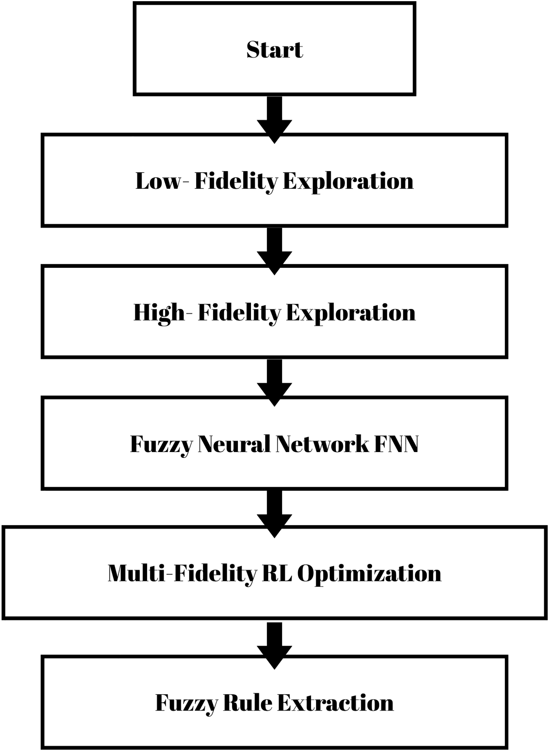
The methodology is built on two pillars: A FNN to deliver interpretable models, and a MFRL strategy to optimize these parameters. The FNN offers the explainability of design decisions, and the MFRL explores the design space efficiently using a family of low- and high-fidelity models. These components interact in an iterative process to explore the design space and find optimal processor configurations as shown in Fig. 2.
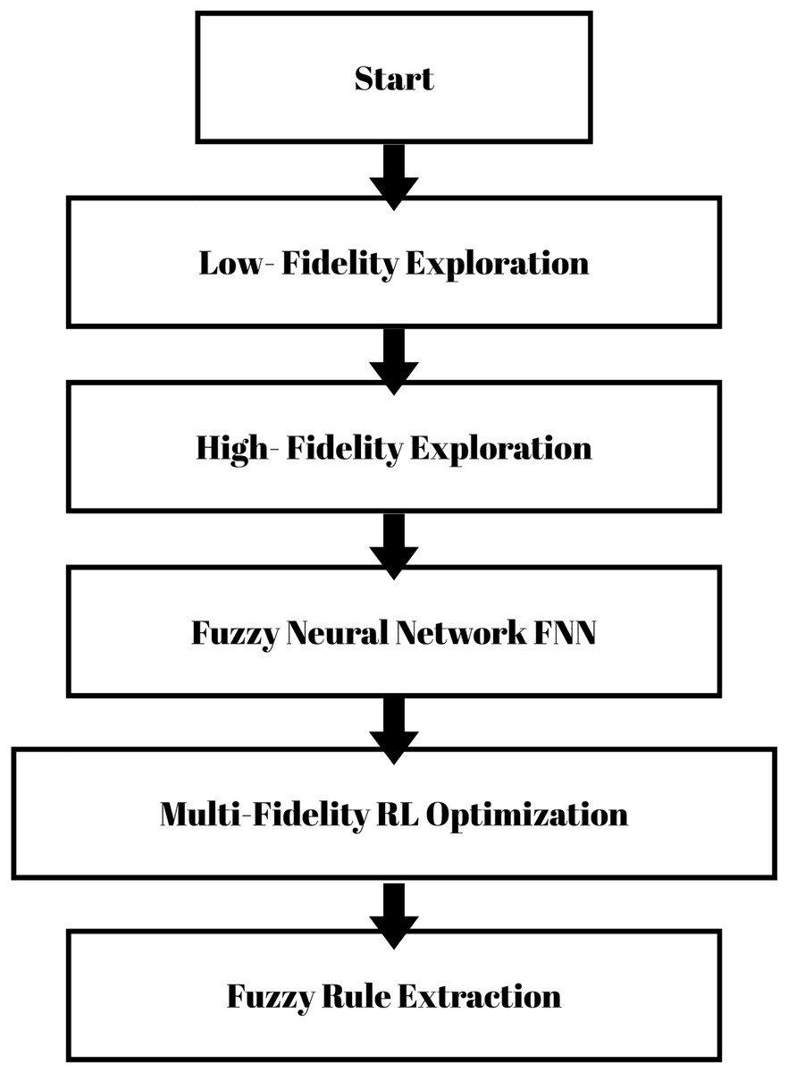
Figure 2: Flowchart of proposed methodology.
Fuzzy neural network
The FRNN enables the interpretability of the optimization process. Fuzzy neural networks can be developed as an extension of a neural network by integrating neural networks, which can adapt their weights, with the transparent nature of fuzzy logic that describes the underlying relationship among the design parameters using fuzzy if-then rules. In this article, we followed the rules of human understanding to clarify the optimization process, providing a mechanistic based explanation which can be applied in terms understandable for the designer and therefore bridging the gap between machine learning models and human-readable design insights.
An FNN model scheme includes an input layer, fuzzy layer and output layer. This synchronous neural article consists of input, hidden and output layers. The fuzzy layer uses fuzzy logic to convert these inputs into fuzzy values processed by the neural network. During classification, the output layer produces human-readable decision rules allowing interpretation of the implications of design parameters on performance outcomes. This set of fuzzy rules facilitates interpretability in the optimised decision making and helps to make optimization paths more visual, as can be seen in Table 4.
FNN architecture details
The model of FNN is composed of three operating layers input, fuzzy, and output. The inputs contain core design parameters: the size of the cache, the depth of the pipeline, and the width of the memory. Use of the triangular membership functions converts crisp input values into fuzzy sets, using the fuzzy layer. Each fuzzy rule has an interpretable format of IF-THEN that links design variables with the performance behavior. This consists of no more than 10 or 15 fuzzy rules so that they may be interpretable. The performance results are constrained to performance such as execution time or power which is mapped by the output layer using fuzzy values. The design assists in producing clear opinions in the process of design optimization.
Multi-fidelity reinforcement learning
The methodology of MFRL evolves the design space effectively. Many approaches are classified as MFRL, which involves a two-phase exploration process wherein the large design regions are first searched quickly at low fidelity and the configurations pointed out in this phase are refined at high fidelity. The framework adopts both types of models to expeditive regulation of the design space exploration and to reduce the number of costly simulations.
The following appropriate basic definition of a Markov decision process is represented under MFRL, where state-space is a processor configuration, and action-space represents the possible changes or optimizations to the design parameters. The reward function is defined over the execution time, power consumption and area performance metrics. The reward mechanism provides feedback to the agent about whether the design it chose was good or bad, guiding the exploration to better configurations. The two-stage consideration is evidenced in Table 5, where the early generations utilize low-fidelity models, while the high-fidelity assessments are performed towards the end for final selection and verification of the design configurations.
| Component | Description | Model type |
|---|---|---|
| State space | Processor configuration parameters | Continuous |
| Action space | Modifications to design parameters | Discrete |
| Reward function | Based on performance, power, and area metrics | Weighted Sum |
RL training
The exploration and exploitation process is balanced using an ε-greedy strategy during the RL training process. In the training, the learning rate is 0.01 with a discount factor of 0.9. Convergence of the training occurs in 500 episodes, which is measured by reward and performance measures. The state space contains coded-processor combos. The actions change one or more design parameters. The reward is a weighted sum of the execution time, area and power penalizing poor trade-offs. This arrangement maintains a stable and consistent learning environment in the design space exploration.
Learning algorithms
Optimum design space and minimum computation time accuracy are based on learning algorithms. This basic framework consists of three major algorithms: Q-learning, Deep Q-Network (DQN), and fuzzy rule extraction from the trained FNN. These algorithms were designed with different goals in optimization process.
Algorithm 1 presents the Q-learning for Multi-Fidelity Exploration, enabling the agent to learn from the design-space interactions exploited to minimize its design costs. Learn the parameters used in Q-learning to find the optimal policy. This algorithm is used in the first low-fidelity exploration phase, when the space of states is massive and we must end up with as few simulations as possible. The agent uses the Q-values to take actions, and updates the Q-values based on each interaction with the design space, as presented in Algorithm 1.
| def Q_learning(state, action_space, reward_function, Q_table): |
| # Initialize Q-table and reward structure |
| for state_action_pair in action_space: |
| Q_table[state_action_pair] = 0 |
| while not convergence: |
| for state in action_space: |
| action = select_action(state) |
| reward = reward_function(state, action) |
| next_state = get_next_state(state, action) |
| update_Q_value(state, action, reward, next_state, Q_table) |
| return Q_table |
The DQN estimates the Q-values using a deep neural network (DNN), enabling it to tackle high-dimensional state space problems. Thus, the network is trained from a replay buffer: a memory of past experiences, so as to stabilize the learning process. Such algorithm is used when it scales the design exploration process to larger and more complex configurations. The DQN is trained iteratively as shown in Algorithm 2, so as to approximate the optimal policy.
| def DQN(state, action_space, reward_function, Q_network): |
| # Initialize deep neural network for Q-value approximation |
| while not convergence: |
| for state in action_space: |
| action = select_action(state) |
| reward = reward_function(state, action) |
| Q_network.update(state, action, reward) |
| return Q_network |
It provides the Fuzzy if-then rules that are extracted from the trained FNN. Thus, generated Convolutional Neural Network (CNN) design rules present interpretable knowledge about the design optimization process, allowing designers to directly see how specific design choices contribute to the performance of their network. A trained FNN model is used to generate human interpretable fuzzy rules, and the process is explained in Algorithm 3.
| def fuzzy_rule_extraction(FNN_model): |
| rules = [] |
| for input_layer in FNN_model.input_layer: |
| rule = generate_fuzzy_rule(input_layer) |
| rules.append(rule) |
| return rules |
Integration of FNN and MFRL
The suggested algorithm has two stages of a two-layer hybrid system that combines FNN and MFRL. The level of simulations has low fidelity in this initial stage, with the Q-learning method being used in fast exploration. The second stage is where the trained configurations are tested on a high-fidelity environment using DQN simulation. In both of the stages, FNN produces human-interpretable fuzzy rules that are used in exploration and also enable designers to interpret decisions. Such an arrangement has increased efficiency and interpretability. The fuzzy rules impact the exploration process and discover relationships among design features as characterized by Table 6.
| Algorithm | Description | Purpose |
|---|---|---|
| Q-learning | Reinforcement learning algorithm used for initial design exploration | Optimal policy learning |
| Deep Q-network (DQN) | Deep learning-based Q-learning for handling large design spaces | Scalable exploration |
| Fuzzy rule extraction | Extracts fuzzy decision rules from the trained FNN | Ensures interpretability |
Evaluation and performance metrics
We demonstrate the effectiveness of our proposed framework by applying it to standard microprocessor design benchmarks. Performance metrics for evaluation are execution time, power consumption, area, and area−delay product. These metrics give a holistic view of design performance and help an agent to make design decisions. As presented in Table 7, the framework optimizes designs based on a weighted sum of these metrics which incentivizes exploration of configurations that reduce execution time (ET) and power consumption (PC) while occupying less area (A).
| Metric | Description | Purpose |
|---|---|---|
| Execution time | Time taken by processor to execute tasks | Performance |
| Power consumption | Energy consumed by the processor during execution | Energy efficiency |
| Area | Physical area occupied by the processor design | Spatial efficiency |
| Area-delay product | Combined metric of area and execution time | Overall efficiency |
The point of comparison in our experiments is a standalone design space exploration process based on high-fidelity simulations and a random parameter search approach. It does not contain learning-based optimization nor explainability. Any type of performance comparison is done to this benchmark based on the aspects of design, speed, and resource consumption.
Results
The outcomes confirm the efficiency of the suggested approach in a number of indicators of processor design. They are execution time, power consumption, area efficiency and area-delay product. We compare all these metrics against our method vs. baseline and alternate configurations. Numerical and graphic evidence is shown in six configuration tables and figures.
The findings are arranged in subsections, each devoted to a performance measure. Optimization 1 is FNN + MFRL. Optimization 2 entails FNN only. Optimization 3 only consists of MFRL. All the results are contrasted with the baseline of Config 1 to Config 5. Complete numerical comparisons are given in Tables 8 to 15.
| Configuration | Execution Time (s) | Baseline | Optimization 1 (FNN + MFRL) | Optimization 2 (FNN) | Optimization 3 (MFRL) |
|---|---|---|---|---|---|
| Config 1: Basic design | 120 | 100% | 90% | 92% | 95% |
| Config 2: Optimized pipelining | 85 | 70% | 60% | 65% | 75% |
| Config 3: Optimized cache | 95 | 79% | 71% | 68% | 82% |
| Config 4: Full optimization | 80 | 66% | 57% | 55% | 70% |
| Config 5: Parallelized design | 75 | 62% | 51% | 59% | 65% |
| Configuration | Power consumption (W) | Baseline | Optimization 1 (FNN + MFRL) | Optimization 2 (FNN) | Optimization 3 (MFRL) |
|---|---|---|---|---|---|
| Config 1: Basic design | 50 | 100% | 90% | 95% | 92% |
| Config 2: Optimized pipelining | 45 | 90% | 80% | 85% | 88% |
| Config 3: Optimized cache | 48 | 96% | 84% | 87% | 89% |
| Config 4: Full optimization | 42 | 84% | 76% | 78% | 81% |
| Config 5: Parallelized design | 40 | 80% | 70% | 75% | 78% |
| Configuration | Area (mm2) | Baseline | Optimization 1 (FNN + MFRL) | Optimization 2 (FNN) | Optimization 3 (MFRL) |
|---|---|---|---|---|---|
| Config 1: Basic design | 75 | 100% | 95% | 96% | 97% |
| Config 2: Optimized pipelining | 70 | 93% | 88% | 90% | 92% |
| Config 3: Optimized cache | 72 | 96% | 91% | 92% | 93% |
| Config 4: Full optimization | 68 | 91% | 84% | 85% | 88% |
| Config 5: Parallelized design | 65 | 87% | 80% | 82% | 85% |
| Configuration | Area-Delay Product (ns·mm2) | Baseline | Optimization 1 (FNN + MFRL) | Optimization 2 (FNN) | Optimization 3 (MFRL) |
|---|---|---|---|---|---|
| Config 1: Basic design | 800 | 100% | 92% | 90% | 85% |
| Config 2: Optimized pipelining | 720 | 90% | 80% | 85% | 82% |
| Config 3: Optimized cache | 780 | 98% | 85% | 87% | 89% |
| Config 4: Full optimization | 700 | 87% | 75% | 76% | 78% |
| Config 5: Parallelized design | 680 | 85% | 73% | 74% | 77% |
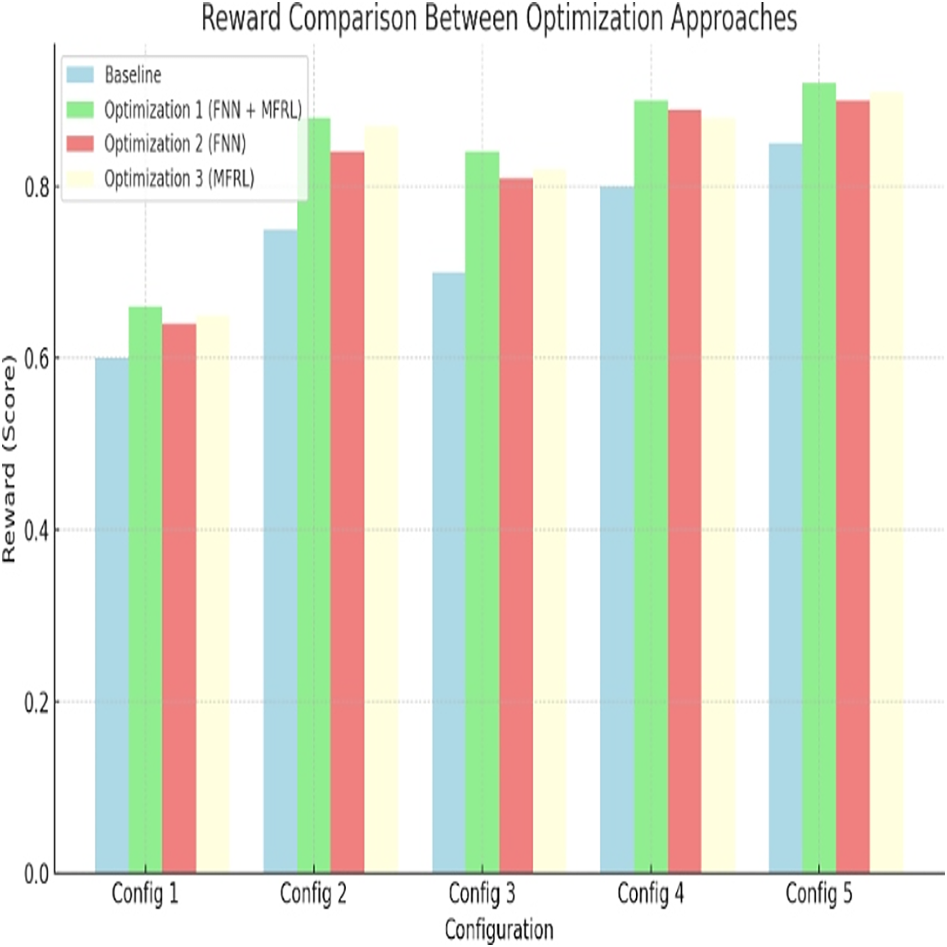
| Configuration | Reward (Score) | Baseline | Optimization 1 (FNN + MFRL) | Optimization 2 (FNN) | Optimization 3 (MFRL) |
|---|---|---|---|---|---|
| Config 1: Basic design | 0.60 | 100% | 110% | 104% | 107% |
| Config 2: Optimized pipelining | 0.75 | 125% | 145% | 140% | 135% |
| Config 3: Optimized cache | 0.70 | 116% | 132% | 129% | 130% |
| Config 4: Full optimization | 0.80 | 133% | 150% | 148% | 146% |
| Config 5: Parallelized design | 0.85 | 141% | 160% | 158% | 153% |
| Configuration | Simulation time (h) | Baseline | Optimization 1 (FNN + MFRL) | Optimization 2 (FNN) | Optimization 3 (MFRL) |
|---|---|---|---|---|---|
| Config 1: Basic design | 5 | 100% | 90% | 85% | 80% |
| Config 2: Optimized pipelining | 4 | 80% | 70% | 75% | 77% |
| Config 3: Optimized cache | 4.5 | 90% | 76% | 72% | 74% |
| Config 4: Full optimization | 3.8 | 76% | 64% | 60% | 65% |
| Config 5: Parallelized design | 3.5 | 70% | 60% | 62% | 64% |
| Configuration | Memory usage (MB) | Baseline | Optimization 1 (FNN + MFRL) | Optimization 2 (FNN) | Optimization 3 (MFRL) |
|---|---|---|---|---|---|
| Config 1: Basic design | 150 | 100% | 90% | 92% | 85% |
| Config 2: Optimized pipelining | 130 | 87% | 80% | 85% | 83% |
| Config 3: Optimized cache | 140 | 93% | 86% | 88% | 89% |
| Config 4: Full optimization | 120 | 80% | 75% | 74% | 78% |
| Config 5: Parallelized design | 110 | 73% | 70% | 72% | 74% |
| Configuration | Search time (h) | Baseline | Optimization 1 (FNN + MFRL) | Optimization 2 (FNN) | Optimization 3 (MFRL) |
|---|---|---|---|---|---|
| Config 1: Basic design | 100 | 100% | 90% | 88% | 85% |
| Config 2: Optimized pipelining | 90 | 85% | 75% | 80% | 77% |
| Config 3: Optimized cache | 95 | 90% | 80% | 83% | 81% |
| Config 4: Full optimization | 85 | 85% | 70% | 68% | 72% |
| Config 5: Parallelized design | 80 | 75% | 65% | 66% | 70% |
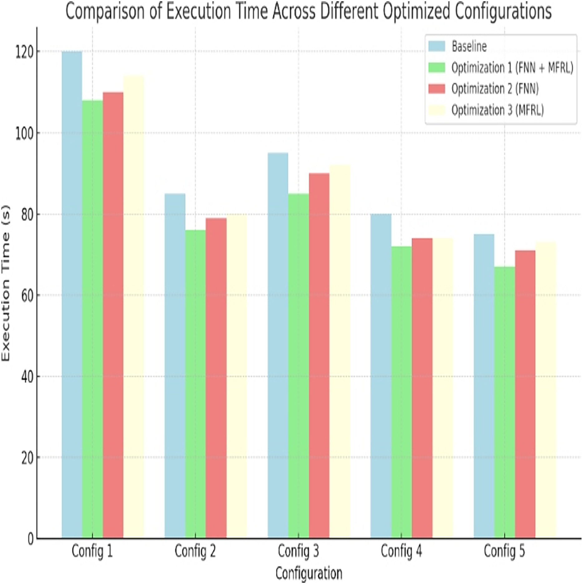
Comparison of execution time
Optimization aims at minimizing the execution time of the processors. All optimized configurations are better compared to gain at baseline. The least overall execution time is provided by optimization 1. In Config 1, there is an improvement of 10 percent. Config 5 does 25 percent better. These are indicated in the Fig. 3 and Table 8. The combination of FNN and MFRL designs the space of designing comprehensively to achieve fast and valid decision-making.
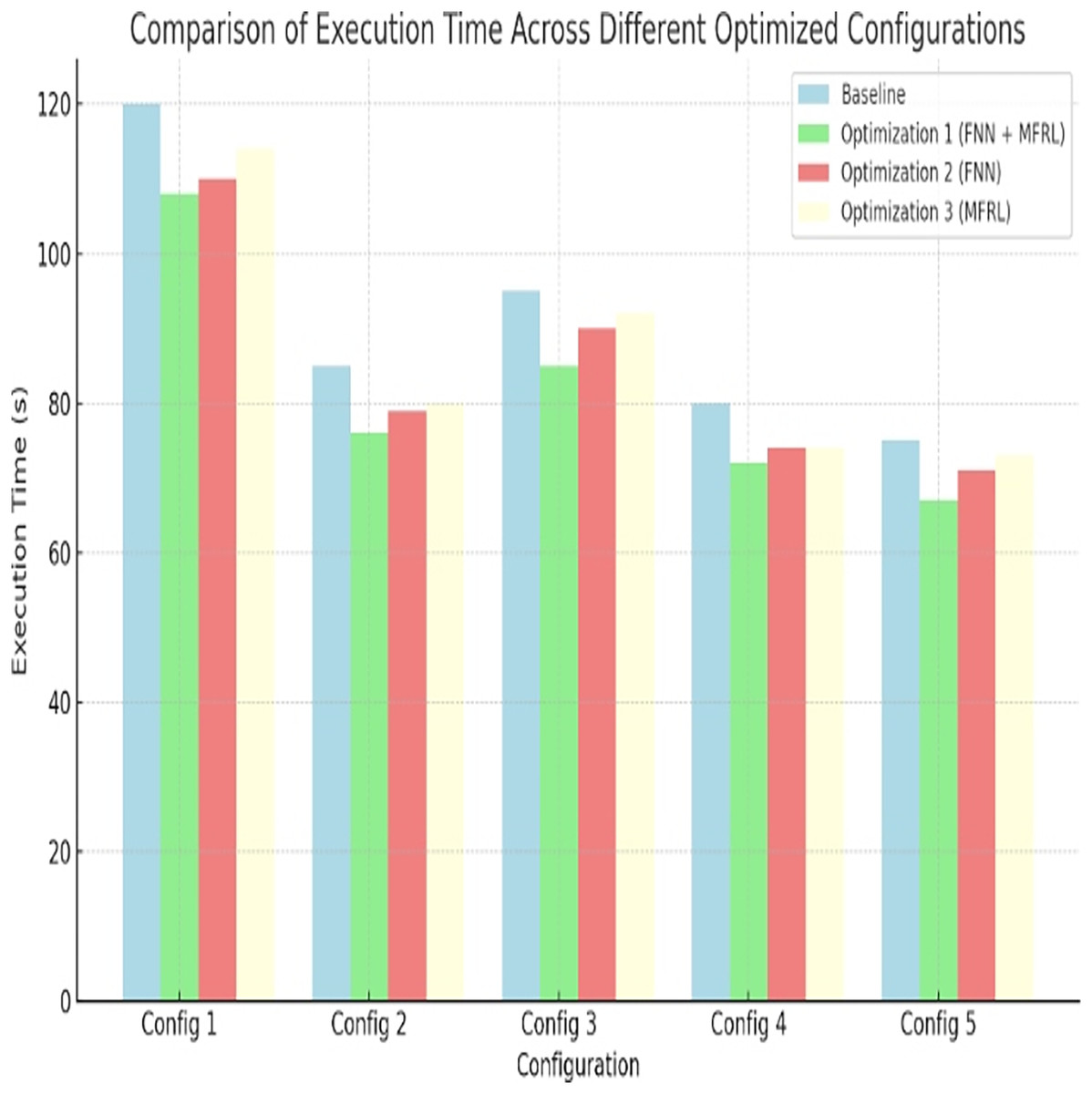
Figure 3: Comparison of execution time across different optimized configurations.
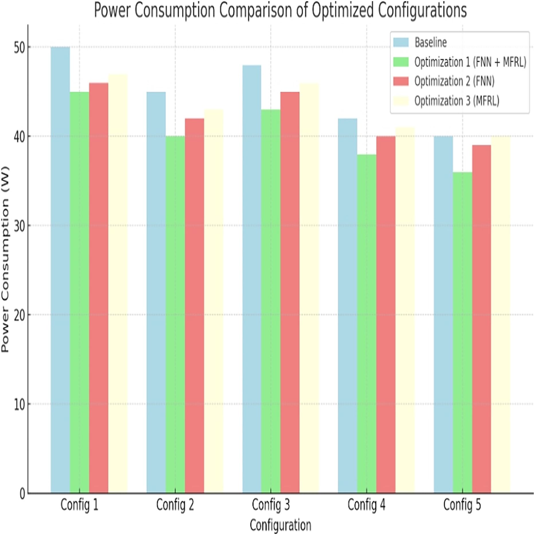
Power consumption: a comparison
Energy is a vital aspect, particularly in embedded systems. Each configuration is lower powered than the baseline. The most significant reduction pertains to Optimization 1, which is 10 percent in Config 1 and 20 percent in Config 5. These reductions are portrayed in Fig. 4 and Table 9. FNN enables power-aware design paths to be refined and MFRL accelerates exploration. A combination of both is better than Optimization 3 because Optimization 1 performs better.
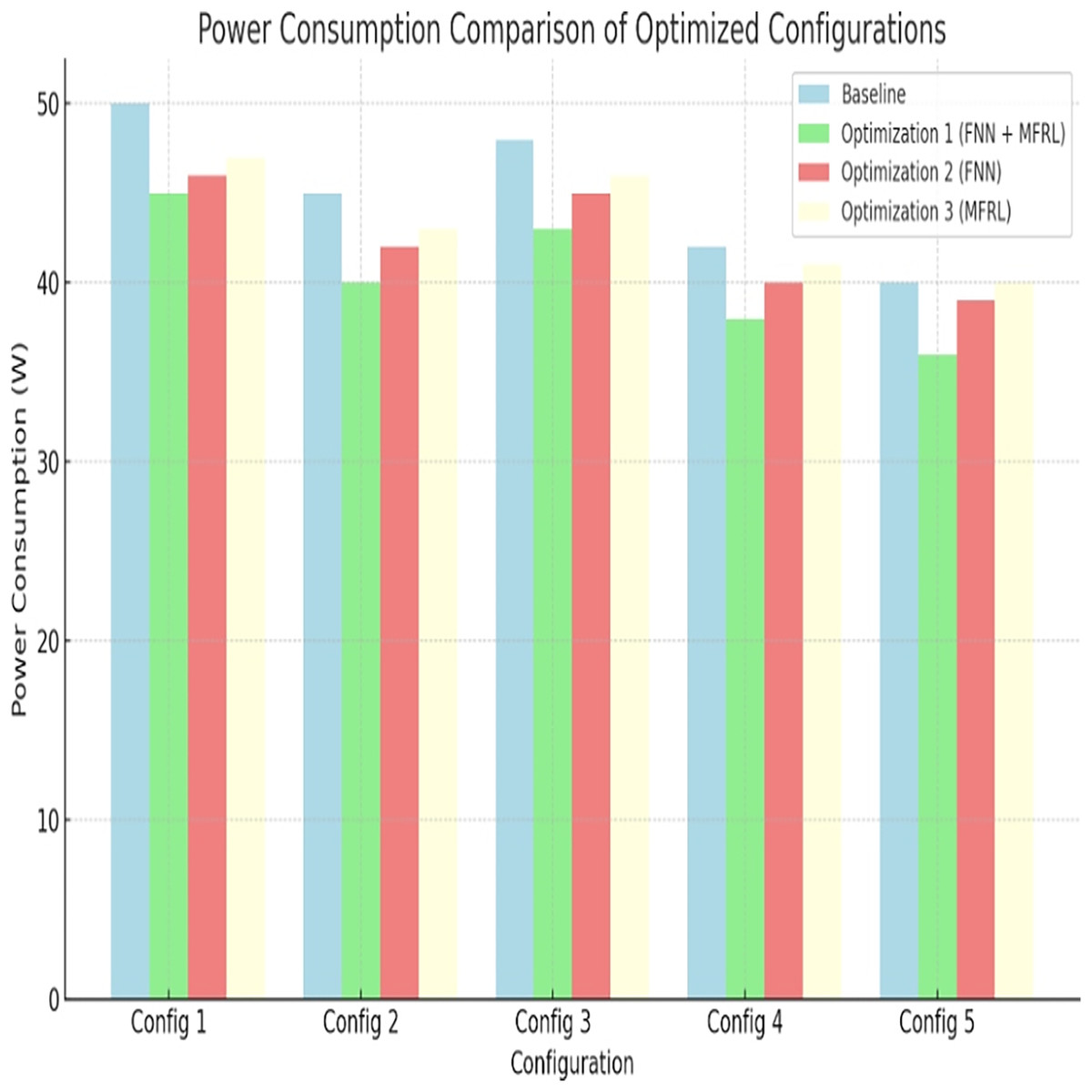
Figure 4: Power consumption comparison of optimized configurations.
Area efficiency
Embedded systems Processor size is important. In terms of area efficiency optimization 1 comes first. Config 1 uses 5 percent area reduction. Config 5 gives 13%. Figure 5 and Table 10 are the results.
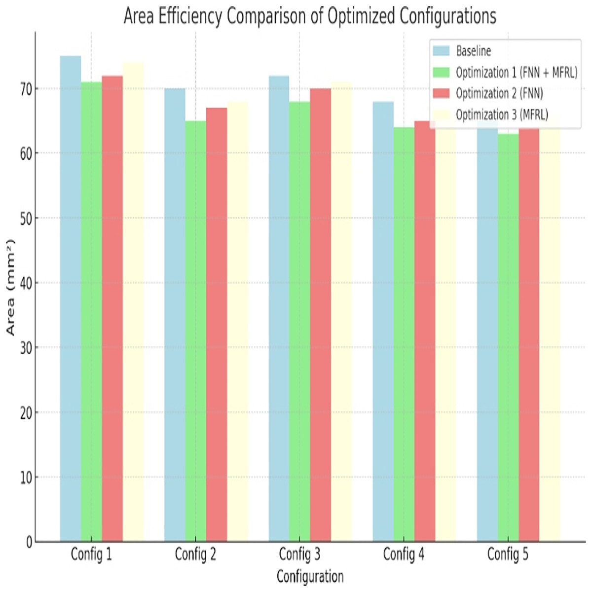
Figure 5: Area efficiency comparison of optimized configurations.
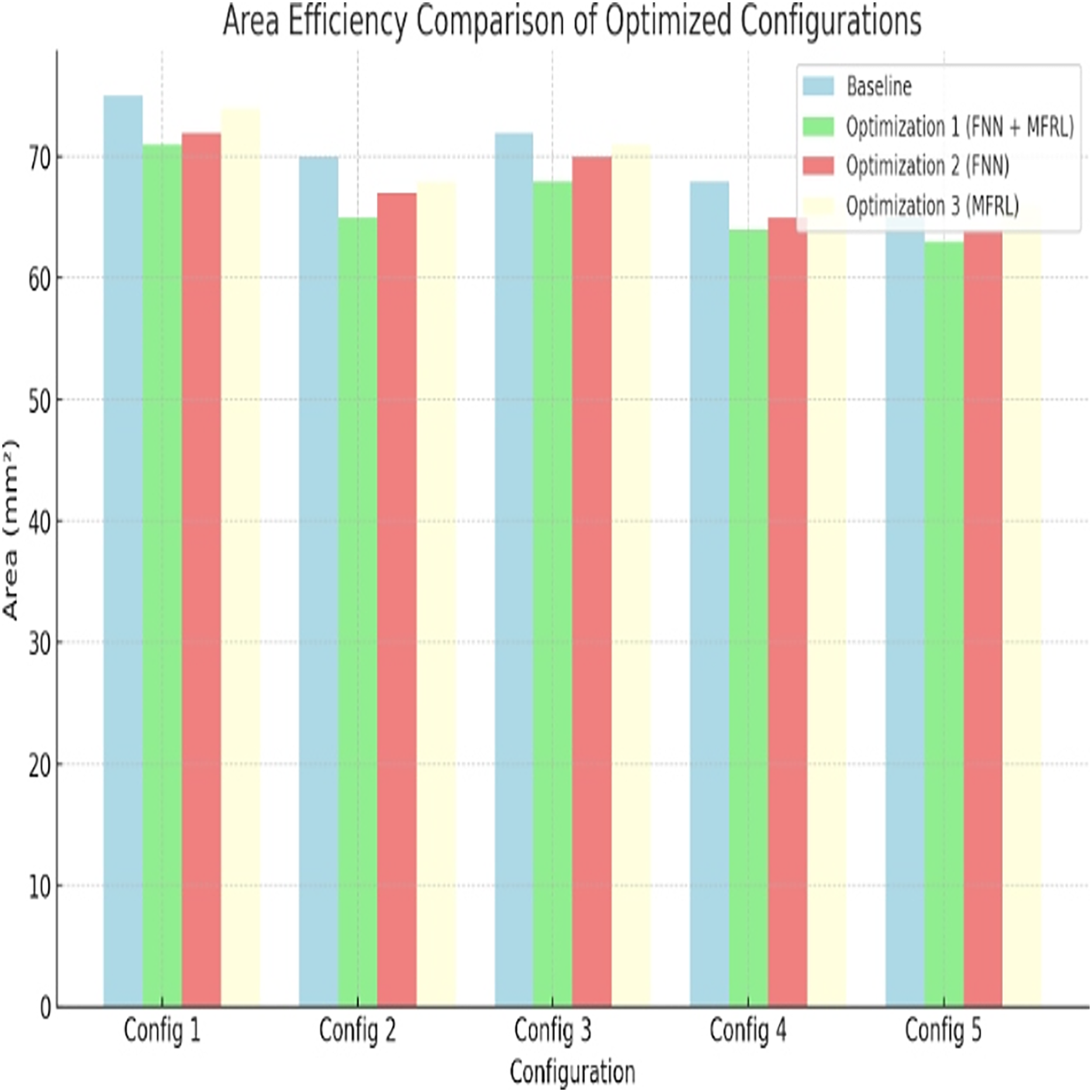
This has been done due to the utilization of fuzzy rules. These are the rules that assist in balancing trade-offs between area and performance. Optimization 2 finds area improvements but those are smaller compared to Optimization 1 that explores more through MFRL.
Area-delay product
Area-delay product is a measure of reasonableness of chip size and speed. A lower the better. Optimization 1 once again works best. It decreases by 12% in Config 1 and by 15% in Config 5. Figure 6 and Table 11 depict the results. This makes it true that the approach results in compact and fast processor designs.
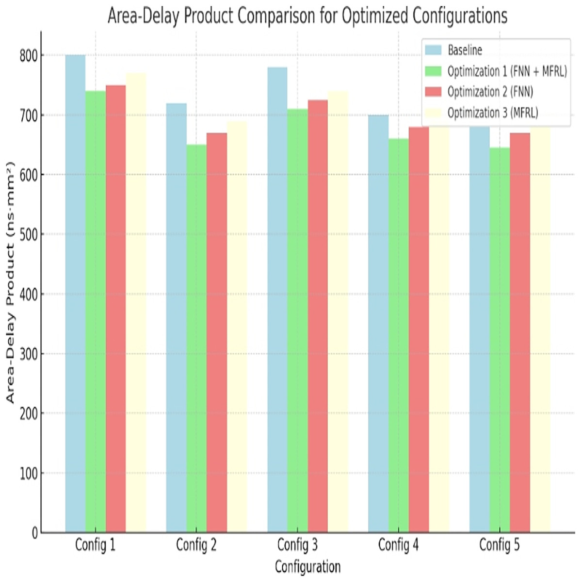
Figure 6: Area-delay product comparison for optimized configurations.
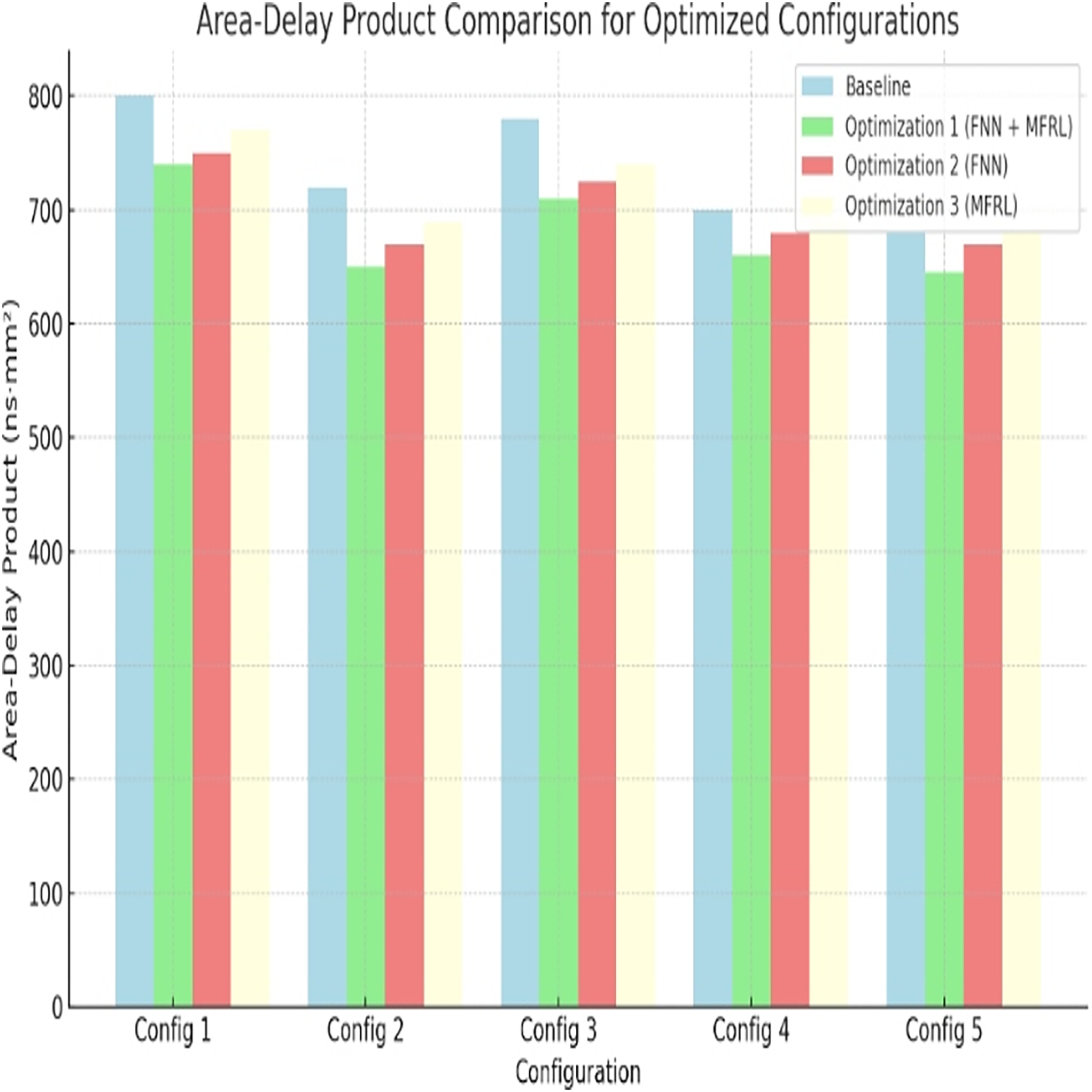
In addition to individual metrics, on the aggregate level, the efficiency is measured on the basis of a composite reward function. This is a combination of power, area and execution time. Greater rewards are signs of improved overall designs. The rewards show balance in trade-offs.
Reward comparison
In every parameter, the highest reward can be seen with Optimization 1. Config 5 has 160 percent better improvement over the baseline. This is confirmed in Fig. 7 and Table 12. FNN and MFRL have a balanced design that outweighs other methods. Optimization 2 and 3 do not have this balance. The suggested approach brings about economic performance in every design dimension.
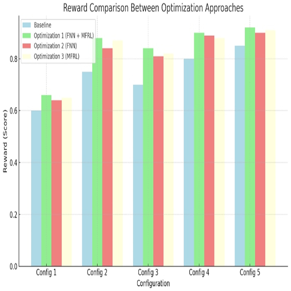
Figure 7: Reward comparison between optimization approaches.
Design time (simulation time) and memory usage
Practical processor design is dependent on design time and memory usage. All the optimization strategies lower simulation time compared with the baseline. The Design time with optimization 1(FNN + MFRL) yields the fastest design time. Optimization 3, too, gives a marked speedup. Table 13 shows these time gains. With regard to memory, the baseline configurations would need less memory than the optimized ones. Optimization 1 performs best as regards memory efficiency. There is a summary Tables 14 and 15 of memory use over configurations. This validates our approach with regard to scalability and practicability.
Discussion
This work proposed a hybrid optimization algorithm that employed explainable fuzzy neural networks and multi-fidelity reinforcement learning. The efficiency of the approach was evidenced in the results of several configurations. There was consistent improvement in execution time, power consumption, chip area and area-delay product. It also produced improved memory and simulation time performance over traditional baselines in terms of methodology.
One of the strongest aspects of this framework is interpretability. Fuzzy rules allow designers to trace the decisions as well as allow them to understand them. This assists in optimizing architectures that do not depend on the black-box models. Multi-fidelity reinforcement learning minimized the number of high-cost simulations used to explore in early exploration. This reduced the time of exploration and the need for resources greatly.
In spite of all these benefits, the methodology presents certain weaknesses. First, the existing fuzzy rule set is hand-crafted and is merely complex. Rescaling this approach to higher architectures can have more rules. It may decrease readability and drag speed of decision-making. Ordinary future research should be in the direction of rule compression or rule pruning.
Second, although reinforcement learning can speed up the exploration process, it is highly reliant on effective hyperparameter settings. Such factors include learning rate, discount factor and reward weights that directly affect the results. This renders the training process sensitive and, at other times, inconsistent among use cases. This dependency would lessen with automating the tuning.
The framework is presently tested against a small benchmarking collection of data. Despite the choice of standard benchmarks that are used, they do not represent all types of processors. There were no general-purpose CPUs or popular large multi-core designs put to the test. This constrains the external accumulation of results. The tests are to be carried out on more granular micro-architectures to build robustness.
The other limitation is on the comparative analysis. The hybrid method was compared with single FNN and MFRL, but none of the common types of optimization, like genetic algorithms or Bayesian optimization or surrogate models, were used to compare the hybrid against them. It is typical of hardware design and gives a wider range of performance. Their inclusion in future comparisons would make the scope of evaluation better.
There is also a matter of scalability. The state space can also go exponentially when the parameters involved in the design increase. This influences how well reinforcement learning and fuzzy rule extraction perform. Even though the framework scales small to medium-sized processors, its behavior with large-scale System-on-Chip (SoC) designs is not yet tested.
The approach does not yet provide any information that gives feedback between the FNN and MFRL levels. After initial integration, each of the components functions in isolation. A feedback loop that is tightly constructed may promote convergence and make the optimization more dynamic. One of the directions is the integration of internet updates of the rules according to the developing reward.
There is also no case study of the real world provided in this work. All these are obtained based on simulated datasets and benchmarks. Using the approach on a commercial processor design would assist in confirming its usefulness. Another issue would be side effects not seen in an artificial setting when deployed in the real world.
It is also with the framework that attention is given just to the static optimization. Dynamic situations like workload changes or power variations are not managed. Real-time embedded systems would be better with the integration of dynamic adaptation.
Finally, the absence of architecture visualization is one disadvantage. The method does not provide a representation of the optimized microarchitecture, although the rules that are produced by the method are interpretable. This feature would enrich the knowledge and increase usability for the hardware engineers.
Conclusion
The current article proposes a compound strategy based on the idea of an explainable FNN and MFRL. This is aimed at maximizing the micro-architecture design and the process also needs to be interpretable. The approach consider the trade-off between effectiveness and effectiveness by employing fuzzy rules and adaptive learning and tiered simulation.
The framework has been observed to be as effective as experimentally proven in several metrics of processor. Optimization 1 (FNN + MFRL) achieved a higher performance in a regular basis as compared to the traditional techniques. It enhanced execution, power consumption, area and area-delay product. Low-fidelity simulations used early in the process were less time-consuming in exploration and the high-fidelity simulations provided accuracy. This trade-off creates better optimization albeit quicker.
The framework optimizes and improves on interpretability. Fuzzy neural networks give understandable rules that are readable by humans. This is the trade off between the black box learning and designer insight. Designers have the ability to negotiate through domain knowledge and transparency of the rule. The process is explained, and such optimization paths are not concealed anymore.
An execution time and power, as well as an area combination is a reward based evaluation. Optimization 1 earned the maximum reward scores above any configuration. This demonstrates the capability of the framework to maximise several measures simultaneously. The fact that FNN and MFRL are synergistic makes it optimize globally, and not local tuning. This design allows strong and scalable hardware.
The framework solves the current shortcomings in micro-architecture style. It is flexible in simple and elaborate set ups. Being both performance and explainability focused, it is futureproof. Future development consists of applying the model into automated design flows. It may also be applied to multicore and heterogeneous platforms. This qualifies it to changing processor technology.