
Towards trustworthy digital health: reliability of uncertainty-aware convolutional neural networks
- Published
- Accepted
- Received
- Academic Editor
- Ka-Chun Wong
- Subject Areas
- Artificial Intelligence, Computer Aided Design, Computer Vision, Data Mining and Machine Learning, Neural Networks
- Keywords
- Digital health, Trustworthiness, Reliability, CNN, Diabetic retinopathy, Melanoma, XAI, Explainability
- Copyright
- © 2026 Di Biasi et al.
- Licence
- This is an open access article distributed under the terms of the Creative Commons Attribution License, which permits unrestricted use, distribution, reproduction and adaptation in any medium and for any purpose provided that it is properly attributed. For attribution, the original author(s), title, publication source (PeerJ Computer Science) and either DOI or URL of the article must be cited.
- Cite this article
- 2026. Towards trustworthy digital health: reliability of uncertainty-aware convolutional neural networks. PeerJ Computer Science 12:e3414 https://doi.org/10.7717/peerj-cs.3414
Abstract
Computer-aided diagnosis (CAD) systems are used in the medical field to assist clinicians in interpreting diseases. CAD can analyze text, audio, and medical images, offering high accuracy and efficiency in medical diagnoses, particularly when employing deep-learning artificial intelligence. However, due to deep learning’s black-box nature, concerns about interpretability and reliability have raised questions about patient and physician confidence in AI-guided clinical diagnoses. As a result, research has increasingly focused on performance and improving trust and transparency. This study proposes a preliminary Trustworthiness Indicator ( ) to quantify reliability and trustworthiness numerically. The Binary Melanoma Detection Classification on dermoscopic images and the Multimodal Diabetic Retinopathy grading problems on ocular fundus images are used to experiment and analyze the behaviors and performance of . The performances were compared with standard metrics to explore potential correlations, weaknesses, and robustness.
Introduction
Integrating Artificial Intelligence (AI) into healthcare can significantly enhance human well-being, thanks to its ability to extract knowledge from data with unmatched speed and precision, often surpassing clinicians in specialized tasks such as image analysis for skin cancer diagnosis (Salinas et al., 2024).
AI now enables the development of diagnostic tools, therapy optimization protocols, and personalized medicine strategies (Chang, 2019; Ghanem, Ghaith & Bydon, 2024). Among these are computer-aided diagnosis (CAD) systems and clinical decision support systems (CDSS), software applications designed to assist healthcare professionals in interpreting medical data and making informed decisions. These systems aim to improve diagnostic accuracy and efficiency by automating analysis tasks (Lembo et al., 2024), providing consistent evaluations, and supporting clinical workflows through alerts and Supplemental Information (Giger & Suzuki, 2008; Ouanes & Farhah, 2024).
CAD and CDSS can process diverse types of medical data and, thanks to advances in Convolutional Neural Networks (CNNs)1 and Vision Transformers (ViTs)2 , have become powerful tools for analyzing medical images3 , including X-rays, CT scans, MRI, mammograms (Staffa et al., 2022), and ultrasound.
Yet, despite their strong diagnostic performance, the trustworthiness of these models remains an open challenge: their black-box nature raises concerns about reliability, uncertainty, and clinical safety.
Existing approaches to trustworthiness in medical AI rely mainly on qualitative assessments or post-hoc explainability methods, such as saliency maps or feature attribution. While these techniques improve interpretability, they do not provide a quantitative and generalizable metric that captures uncertainty and robustness across diverse clinical contexts.
This gap motivates our work. We introduce a Trustworthiness Indicator ( ) designed explicitly for uncertainty-aware CNNs in digital health applications. Unlike post-hoc Explainable Artificial Intelligence (XAI) methods such as SHapley Additive exPlanations (SHAP) or Local Interpretable Model-Agnostic Explanations (LIME), which explain individual predictions through feature attribution, quantifies the consistency of internal representations across models. In this way, complements interpretability metrics by providing a measurable assessment of reliability that is essential for clinical trust.
From a clinical perspective, could be integrated into CAD or CDSS as a reliability layer accompanying standard outputs. Alongside the predicted diagnosis and associated saliency maps, a CAD system could display the score to indicate the level of consistency in the model’s internal reasoning. A high value would reassure clinicians that the prediction is based on stable feature representations. At the same time, a low score would signal caution and potentially prompt a second opinion or further examination. Thus, does not replace clinical judgment but provides actionable information on model robustness, fostering informed trust in AI-assisted decision-making.
The role of AI in improving diagnostic processes
Machine learning (ML) and deep learning (DL) can analyze vast amounts of medical data, including images, patient records, and genetic information, to assist healthcare professionals in identifying diseases and conditions with greater precision. These technologies excel in image-based diagnostics, where AI models can detect patterns in medical imaging data, such as X-rays, MRIs, or pathology slides, that may be imperceptible to the human eye. In addition to improving diagnostic accuracy, AI enables early detection of diseases, personalized treatment plans, and reduced human error. As AI continues to evolve, its role in healthcare is expected to grow, offering the potential to revolutionize diagnostic processes and enhance patient outcomes across various medical specialties.
Figure 1 reports images related to Melanoma and Diabetic Retinopathy, two diseases used in this work as a real CAD scenario.
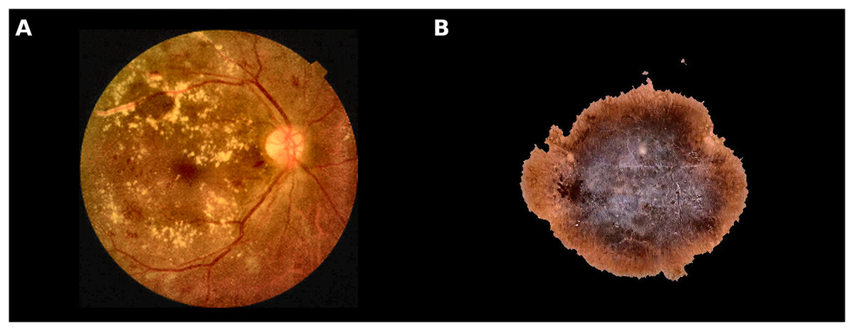
Figure 1: Examples of different classes used in this study.
(A) Retina shows microaneurysms, haemorrhages, and exudates; (B) Malignant skin lesion (Melanoma).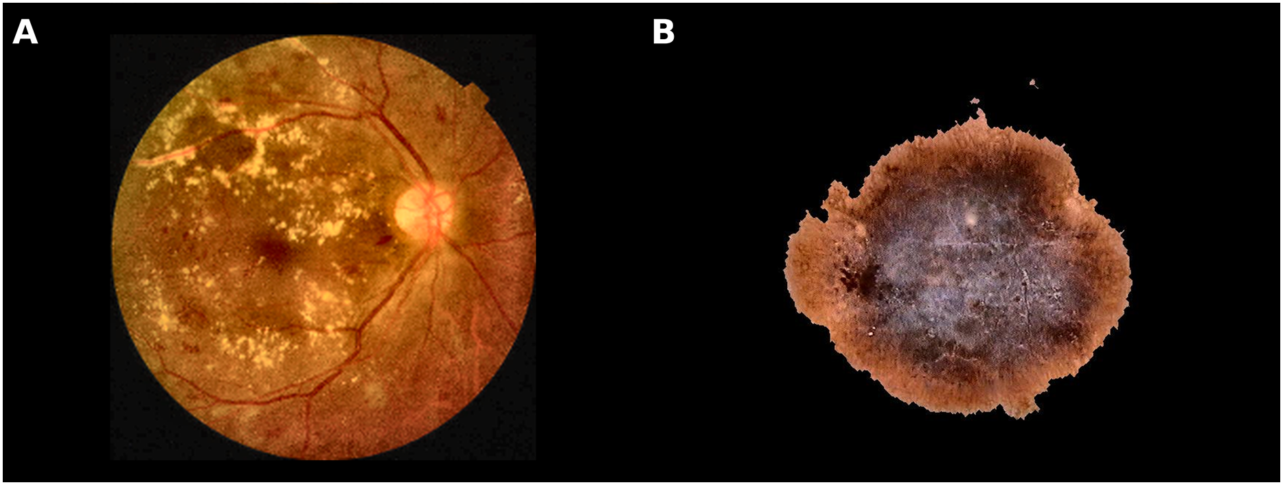
Improving melanoma detection through artificial intelligence
Melanoma is a skin cancer originating from transformed melanocytes (Brunsgaard, Jensen & Grossman, 2023)4 into tumor cells. Diagnosing and managing malignant melanoma involve a combination of methods, including the manual examination of dermoscopic images, biopsy, histopathological analysis, and sometimes imaging techniques for determining the cancer stage. Physicians often rely on established diagnostic criteria, such as the ABCDE rule, which assesses asymmetry, border, color, diameter, and evolving changes in a lesion (Duarte et al., 2021). Since melanoma can evolve, routine medical monitoring is essential to detect suspicious skin cell changes (Brunsgaard, Jensen & Grossman, 2023). In modern practice, the repetitive and routine task of monitoring skin lesions—which is prone to human error (Reason, 1995)—can be efficiently carried out by AI-based tools (Brodeur et al., 2024).
Addressing malignant melanoma requires a proactive approach and precise early diagnosis: Early intervention and treatment significantly reduce the risk of death associated with melanoma (Rigel & Carucci, 2000). Conversely, slow or inaccurate intervention can significantly increase life-threatening risks. While a false positive diagnosis is generally acceptable, a false negative diagnosis can have severe, life-threatening consequences (Di Biasi et al., 2022).
Papachristou et al. (2024) evaluated AI performances in a real-life clinical trial. The authors evaluated the performance of an AI-based clinical decision support tool for detecting cutaneous melanoma, operated through a smartphone app. The authors want to demonstrate whether AI could provide substantial clinical value for primary care physicians assessing skin lesions for melanoma. The study involved 253 lesions from 228 patients, 21 of which were melanomas, including 11 invasive and 10 in situ melanomas. The app achieved an impressive diagnostic accuracy, with an area under the receiver operating characteristic (AUROC) curve of 0.960 (95% CI [0.928–0.980]), yielding a maximum sensitivity of 95.2% and specificity of 84.5%.
Heinlein et al. (2024) performed an “All Data are Ext” experiment comparing the diagnostic accuracy of AI and dermatologists on a prospectively heterogeneous test set comprising distinct hospitals, different camera setups, rare melanoma subtypes, and special anatomical sites. The results show that the AI achieved higher balanced accuracy than dermatologists, with a higher sensitivity at the cost of lower specificity. The authors concluded that, as the algorithm exhibits a significant performance advantage on the heterogeneous dataset exclusively comprising melanoma-suspicious lesions, AI may offer the potential to support dermatologists, particularly in diagnosing challenging cases.
Strzelecki et al. (2024) reviewed many applications of different AI algorithms for melanoma detection, both classic systems based on the analysis of dermatoscopic images and total body systems. Results of the review strongly suggested that AI can obtain results comparable to the assessment of specialists. According to the authors, AI is increasingly valuable in dermatologic diagnostics and other medical fields. However, for successful AI integration, physicians need a solid understanding of AI, including its limitations and the reasoning behind decisions made by explainable AI. Still, challenges remain, including technical issues like ensuring access to high-quality medical data and legal issues such as creating clear rules for AI use in clinical practice.
Artificial intelligence and diabetic retinopathy disease
Diabetic retinopathy (DR) is a serious complication of diabetes mellitus caused by prolonged periods of inadequately controlled blood sugar. If not appropriately managed, DR progressively damages the blood vessels of the retina, causing vision damage (Fong et al. 2003), sometimes irreversible (Kusuhara et al., 2018). DR advances through several stages: It first manifests with mild non-proliferative changes (NDPR), characterized by increased permeability of the retinal blood vessels. Subsequently, with the passage of time and the progression of the disease, it progresses to a moderate to severe non-proliferative stage, characterized by a closure of the blood vessels, causing limited blood supply to the retina. In the more advanced stage, proliferative diabetic retinopathy (PDR), new abnormal blood vessels develop on the retina’s surface and in the posterior part of the vitreous body (Yang et al., 2022). Also, macular edema5 can occur at any stage of retinopathy (Fong et al., 2004).
According to Salz & Witkin (2015), clinicians can perform various examinations to diagnose DR, such as color fundus photography, fluorescein angiography (FA), B-scan ultrasonography, and optical coherence tomography (OCT). Images obtained through previous techniques can reveal various abnormalities caused by DR, such as red lesions like microaneurysms (MAs)6 and intra-retinal hemorrhages (HMs). In addition to these, white lesions associated with DR include exudates (EXs)7 and cotton-wool spots (CWSs)8 (D’Amico, Shah & Trobe, 2023). The correlation between the visual examination of the ocular fundus and the detection and grading of DR has led to the proposal of various machine learning and deep learning models for DR detection and grading, mainly using CNN, a network architecture capable of extracting classification and prediction features unsupervised.
Qummar et al. (2019) proposes a hybrid approach for the detection and classification of DR using GoogleNet to capture spatial and local features of retinal images and ResNet-16 to mitigate the vanishing gradient problem and improve classification accuracy, combined with the Adaptive Particle Swarm Optimizer (APSO) for feature extraction optimization. The features extracted from the two models are merged into a vector of 2,000 features, which is then classified using various machine learning algorithms (Support Vector Machine, Random Forest, Decision Tree, Naive Bayes). The dataset used is EyePACS, consisting of more than 35,000 images of the ocular fundus, divided into five classes of DR severity. The model’s performance was measured in accuracy, precision, recall, and F1-score. The model with the best overall performance was the Radial SVM with an accuracy of 94%, precision of 97%, F1-score of 96%, and recall of 89%.
Mutawa, Alnajdi & Sruthi (2023) explored the use of transfer learning for detecting DR, analyzing, in particular, the effectiveness of combining multiple datasets to improve the generalization of DL models. The authors use four pre-trained CNNs (VGG16, InceptionV3, DenseNet121, and MobileNetV2). Three datasets were used to train and test the models: APTOS, EyePACS, and ODIR. The models were first evaluated on the singular datasets and then on their combination. The results show that the overall performance of the deep learning models improves when trained and tested on a combined dataset, compared to when they operate on single datasets. Specifically, the DenseNet121 model obtained on the combined dataset an Accuracy of 98.97%, Precision of 98.97%, Recall of 98.97% and Specificity of 99.48%, while on the individual datasets, it reported APTOS: Accuracy 98.50%, Precision 98.50%, Recall 98.50%, Specificity 98.50%, EyePACS: Accuracy 89.10%, Precision 89.10%, Recall 89.10%, Specificity 89.10%, ODIR: Accuracy 75.82%, Precision 75.82%, Recall 75.82%, Specificity 75.82%.
Thomas & Jerome (2024) proposes an approach based on transfer learning and ensemble learning for detecting and classifying DR, exploiting a hybrid model consisting of three CNN networks working in parallel and an SVM classifier. The dataset includes ocular fundus images from Messidor, EyePACS, and an in-house clinical dataset. The proposed model obtained a model accuracy of 98%, Precision 98.99%, Recall 99.78%, F1-score 99.38%, MCC 95.53%, and Jaccard Index 95.5%. The results confirmed that an ensemble approach with multiple CNNs and SVM can improve accuracy in the classification and detection of DR.
Abdulateef (2025) proposed a multi-sequence attention framework for brain tumor classification, integrating CNNs with Grad-CAM and SHAP to enhance both accuracy and transparency in medical imaging.
The rising need for trustworthiness in AI in digital health
The high and increasing accuracy, together with the growth of AI in the Digital Health field, leads to a growing interest in determining how reliable the answers to these methods are from a clinical point of view. Recent studies highlight the growing interest of the scientific community in trust in AI systems in the healthcare domain, increasingly considering it a key factor for clinical adoption, on par with technical performance. In particular, Hassija et al. (2024) emphasize that AI must be implemented reliably and transparently for trust and ethical clinical decisions.
Helenason et al. (2024) investigated the feasibility of an AI-based CDSS to detect cutaneous melanoma in primary care. The results demonstrated that an AI-based CDSS could play an important role in cutaneous melanoma diagnostics due to sufficient evidence of diagnostic accuracy. However, the reports from the interviews with fifteen primary care physicians revealed that trust in the CDSS emerged as a central concern. Interestingly, scientific evidence supporting the diagnostic accuracy of the CDSS was identified as a key factor that could increase trust.
Fosso Wamba & Queiroz (2023) highlight the growing role of responsible AI9 in digital health, stressing the need for trustworthiness and ethical integrity. Privacy concerns, ethical issues, and cultural resistance are key barriers to AI adoption. Responsible AI approaches help address medical tensions, particularly in data privacy and governance. Publication trends and emerging technologies further support the necessity of ethical and high-performing AI systems (Reinhardt, 2023).
According to Laux, Wachter & Mittelstadt (2024), due to the black-box nature of AI models, patient and physician confidence in diagnosis and treatment is essential in every guided AI-clinical diagnosis; therefore, tackling the lack of transparency in these AI models becomes essential for researchers to encourage ongoing collaborations between AI developers and clinical end users. The author’s conclusion highlights the importance of transparency and participatory approaches in building trust, especially in sectors like healthcare. Also, the authors highlight how trust research remains fragmented and how further research and sector-specific regulation are necessary to address the complexities of trust in AI, ensuring that institutions and intermediaries play a key role in fostering trust and transparency in AI-driven clinical decisions.
In this evolving scenario, ethical considerations, including consent, explainability, and fairness, have played a central role in designing AI systems, effectively becoming key aspects to be considered “by design” in their development and implementation. For example, future AI models in Europe must follow the “do not harm” rule (https://artificialintelligenceact.eu/article/5/) and align with the EU Parliament’s recommendation. Additionally, they must adhere to principles of transparency10 , ensuring that AI systems are transparent and their decision-making processes are understandable to users. Fairness must also be a central consideration, ensuring that AI models “do not harm” (discriminate) and operate equitably across different populations. These requirements aim to promote trust, accountability, and ethical responsibility in AI systems, aligning with broader legal and ethical standards that govern their deployment in various sectors, including healthcare, to safeguard public well-being. If we agree with the previous observations and results, it is reasonable to state that guaranteeing interpretability, explainability, and trustworthiness will be essential for future AI systems in healthcare, alongside other key aspects such as performance, robustness, and ethical considerations. Therefore, this contribution aims to stimulate discussion on the need for a quantitative definition of “trustworthiness”. We argue that this indicator should be defined to support the development of all future healthcare AI-based applications.
Consequently, we propose a raw definition of this Trustworthiness Indicator ( ), applied to two specific CAD scenarios: the Melanoma Binary Classification Problem (MBCP), and to Diabetic Retinopathy Classification and Grading (DRCG), introduced in brief in the following sections. These problems help us investigate ( ) properties in scenarios that cover image processing aspects of the AI-CAD system in healthcare.
Finally, we discuss future works and the limitations of our current proposal. In particular, we highlight the need to understand whether this indicator should be used alongside classical performance metrics, such as accuracy and precision, or whether it could serve as a stand-alone indicator, which requires deeper investigation. Moreover, beyond images, future work should also consider the importance of purely numerical analyses, as they could provide valuable insights in complement to visual data.
Explainability, interpretability (XAI), and uncertainty in AI for healthcare
Decisions in healthcare carry ethical and psychological implications. They could profoundly impact patient well-being and life because they can determine the accuracy of diagnoses and the effectiveness of treatments11 . Timely decision-making is also critical, as delays can worsen conditions, reduce survival chances, and compromise the overall safety of medical interventions. Therefore, if we want to use AI in digital health, it is reasonable to consider it crucial to ensure that AI systems are transparent, interpretable, explainable, and ethically designed to support accurate diagnoses, effective treatments, and patient safety while maintaining trust and minimizing potential risks.
Interpretability refers to how easily a human can understand the internal workings of an AI model12 . It focuses on how inputs relate to outputs, even if the reasoning process is not explicitly stated. It explains why a model made a specific decision. For example, Grad-CAM highlights which part of an image influenced the classification of a CNN (Selvaraju et al., 2020).
Explainability refers to the degree to which AI systems can clearly articulate their decision-making processes. The AI system can provide understandable reasons for its decisions, often involving the generation of human-friendly explanations for complex or ‘black-box’ models like deep learning networks.
Unfortunately, defining trust is challenging. Consider a CNN model used to classify medical images. If Grad-CAM highlights irrelevant regions while the model still achieves high accuracy, the model is interpretable but not trustworthy. On the other hand, consider a CNN that consistently provides accurate and well-calibrated diagnoses but functions as a “black box” without clear explanations. In this case, the model is trustworthy but not interpretable.
According to Starke & Ienca (2024), many forms of trust in AI exist, and the deep learning-based applications preclude comprehensive human understanding. Nevertheless, trustworthiness refers to how reliable, robust, and safe the AI system is across different conditions. It assesses whether a model’s outputs can be depended upon. For example, a well-calibrated confidence score (e.g., via temperature scaling) ensures that when the model predicts “90% confidence,” the actual correctness is close to 90%.
Table 1 summarises the distinction between XAI and trustworthiness. XAI focuses on making AI decisions understandable, while trustworthiness ensures robustness and reliability essential for clinical adoption.
| Feature | XAI | Trustworthiness |
|---|---|---|
| Purpose | Helps humans understand why AI made a decision | Ensures AI decisions are reliable and robust |
| Key techniques | Grad-CAM, SHAP, LIME, Feature Attribution | Uncertainty Estimation, Calibration, Robustness Testing |
| Main users | Clinicians, AI developers | Uncertainty Regulators, Healthcare Providers |
| Example in medical AI | Explaining why a model labeled a skin lesion as melanoma | Ensuring the model does not fail unpredictably on new patient data |
If we integrate AI into the healthcare field and accept that decisions in healthcare can profoundly impact patient outcomes, healthcare providers and patients must understand how AI arrives at its recommendations. If an AI system functions as a “black box’ offering little insight into the rationale behind its decisions, skepticism and hesitation in adopting the technology are likely: this is particularly concerning in healthcare, where the stakes are high, and errors can have severe consequences.
According to Gille, Jobin & Ienca (2020), clinicians need confidence in their ability to interpret AI-generated insights effectively (and they must not see AI as concurrent), while patients require clear explanations of treatment options influenced by AI and, to earn trust, healthcare AI must undergo rigorous validation and testing to ensure accuracy, safety, and performance across diverse populations and medical conditions. Additionally, according to Kundu (2021), healthcare AI must be explainable, and its explanations must have clinical relevance.
As reported by Saraswat et al. (2022), the XAI research field provides multiple techniques to help understand the decision-making processes of complex artificial intelligence models, providing insights into the factors contributing to their outputs, allowing users to verify and validate the reasoning behind AI decisions: this aspect may lead to increased trustworthiness in AI system in digital health. Also, according to Hassija et al. (2024), XAI can make AI more accessible, reliable, and trustworthy in clinical settings.
XAI and trustworthiness in melanoma classification problem
Focusing on MBCP, many works have focused on using XAI in melanoma detection to improve diagnostic accuracy and confidence and collaboration between AI systems and healthcare professionals, providing transparency and interpretability. Following, we provide studies on applying the Grad-CAM algorithm on melanoma and skin datasets to improve trustworthiness.
Nunnari, Kadir & Sonntag (2021) used VGG16 and ResNet50 classifiers on a dataset comprising 2386 RGB skin lesion images accompanied by five ground truth feature maps, aiming to quantify the extent to which thresholded Grad-CAM saliency maps can effectively highlight visual features associated with skin cancer. The overall accuracy for VGG16 and ResNet50 was observed to be 72.2% and 75.3%, respectively.
Gamage et al. (2023) employed the XCeption model on the HAM10000 dataset, reaching a classification accuracy of 90.24%. Their study involved retaining batch-normalization layers and utilizing Bayesian hyperparameter search for fine-tuning, contributing to the model’s robust performance. To enhance the interpretability of the classification model, the authors introduced the generation of heatmaps using Grad-CAM and Grad-CAM++. These heatmaps offer a visual representation that explains the contribution of each input region to the final classification result.
Li et al. (2024) presented the Uncertainty Self-Learning Network (USL-Net), an innovative method that removes the requirement for manual labeling guidance in segmentation tasks. The procedure starts with extracting features via three contrastive learning methods and then generating Class Activation Maps (CAMs) that operate as saliency maps. Experimental validation on ISIC-2017, ISIC-2018, and PH2 datasets showed that USL-Net performs similarly to supervised methods and outperforms other unsupervised approaches.
According to Wu et al. (2024), extracting data-efficient features from images using Grad-CAM is challenging because models often take shortcuts to complete the task, such as classifying based on meaningless features (non-data-efficient features) like hospital logos. The authors proposed a methodology to mask meaningless features that affect classification and tried to guide the prediction of the classification model based on data-efficient features to improve the performance of various segmentation networks for melanoma detection. Our proposal recalls these findings when we hypothesize that activation pattern consistency among diverse models and high consensus in prediction may indicate model robustness, generalizability, and trustworthiness.
XAI and trustworthiness in diabetic retinopathy problem
In Jiang et al. (2020) the authors propose a method for the classification of diabetic retinopathy using pre-trained CNNs (Inception-V3, ResNet-50 and DenseNet-121), applying the transfer learning technique to adapt them to the specific task of diabetic retinopathy classification and a Grad-CAM-based interpretability technique to generate the activation maps that highlight the regions of the images that most influence the model’s decisions. The dataset used for training and testing the model is APTOS. The best architecture, DenseNet-121, achieved 93% accuracy in classifying the different stages of DR, while the maps generated by Grad-CAM showed that the model correctly focuses attention on relevant retinal lesions such as microaneurysms and haemorrhages.
In Heisler et al. (2020) the authors explore the use of CNN (VGG19, ResNet50 and DenseNet) for the classification of diabetic retinopathy, through the use of Optical Coherence Tomography Angiography (OCTA), integrating Grad-CAM to highlight the most influential image regions in the classification of DR. Grad-CAM made it possible to generate visual activation maps, showing the areas of the OCTA images that had the most significant impact in the model’s predictions, allowing microvascular structures and abnormalities in the deep capillary plexus to be highlighted, indicating the most significant regions for classifying DR by increasing the transparency of the model, reducing the problem of uninterpretable decisions typical of CNNs.
In Quellec et al. (2021) the authors propose ExplAIn, an explainable artificial intelligence (XAI) model for the diagnosis of RD based on deep learning, with the purpose, not only to classify ocular fundus images, but provides visual and textual explanations for its decisions, intending to try to overcome the black-box nature of deep learning models. The model is trained to automatically distinguish lesions from the healthy part of the retina, modifying the input image by simulating lesion removal, turning it into a healthy eye. The CNN learns to automatically identify the presence and severity of DR, classifying images according to the stages of the disease. The Grad-CAM technique generates activation maps to highlight the regions of the image most relevant for classification. Finally, the model produces textual explanations in addition to the visual maps, clearly indicating the identified lesions and their influence on the final decision.
The role of uncertainty in AI trustworthiness in the digital health field
In clinical applications, decisions can significantly impact patient outcomes. Therefore, we argue that quantifying uncertainty is crucial for assessing the reliability and trustworthiness of AI models. Traditional uncertainty quantification (UQ) techniques follow multiple approaches, with Bayesian and ensemble-based strategies being among the most widely used (Abdar et al., 2021).
Bayesian techniques—such as Monte Carlo (MC) Dropout, Markov Chain Monte Carlo (MCMC), and Variational Inference (VI)—utilize probabilistic frameworks to estimate the posterior distributions of model parameters, providing a measure of uncertainty inherent in the model’s predictions (Schoot et al., 2021).
Ensemble methods, including Deep Ensembles and Dirichlet Deep Networks, aggregate outputs from multiple independently trained models to evaluate prediction variance, offering a complementary perspective on model reliability. Additionally, alternative techniques, such as evidential deep learning and adversarial robustness analysis, are gaining traction in uncertainty quantification (Mohammed & Kora, 2023).
Each approach has its strengths and limitations. While theoretically sound, Bayesian methods can be computationally demanding and require careful tuning. Ensemble approaches enhance robustness but may struggle to fully separate epistemic uncertainty (stemming from model limitations) from aleatoric uncertainty (arising from inherent data variability). Moreover, commonly used confidence measures, such as softmax probabilities, primarily reflect aleatoric uncertainty and, if uncalibrated, may lead to overconfident predictions in specific high-risk applications. However, various calibration techniques, such as temperature scaling, can help mitigate this issue.
In the field of digital health, studies have increasingly focused on the role of uncertainty quantification as it directly influences clinical decision-making.
Hassan & Ismail (2025) proposes Bayesian Deep Learning (Bayesian DL) methods. Bayesian approaches provide a way to quantify uncertainty by estimating the posterior distributions of model parameters. Lee & Kim (2022) presents a Bayesian CNN approach with Monte Carlo dropout sampling for metabolite quantification in proton magnetic resonance spectroscopy, enabling simultaneous uncertainty estimation in the predictions.
Gawlikowski et al. (2023) shows that progress in quantifying uncertainty in AI models and its application in digital health remains hindered by standardization, ground truth validation, pointwise evaluation, and explainability challenges. Also, the authors state in their review that addressing these challenges is essential to increasing trust and adoption of AI in healthcare, where uncertainty quantification plays a crucial role in ensuring safe and accurate outcomes.
Abdulateef (2025) proposed a multi-sequence attention framework for brain tumor classification, integrating CNNs with Grad-CAM and SHAP to enhance both accuracy and transparency in medical imaging. The author report that the proposed model achieved an F1-score of 0.97 and an AUC of 0.98, outperforming baseline CNNs (F1 = 0.88) and radiomics-based SVM models (F1 = 0.84). It is worth mentioning that interpretable saliency maps overlap with expert annotations with up to 90%. Therefore, the framework not only improved predictive performance but also suggested a potential increase in clinicians’ trust, as indicated by a reported mean interpretability rating of 4.8/5.
Although Deep Neural Networks (DNNs) have significantly advanced medical image analysis, many models struggle to properly quantify uncertainty in their predictions, especially in complex and noisy real-world environments. This limitation reduces their reliability, particularly in healthcare, where uncertainty in AI decisions can directly impact patient outcomes. A significant issue is the lack of established ground truth uncertainty, making comparing different uncertainty quantification methods difficult.
Authors’ findings emphasize how a standardized evaluation protocol prevents broader adoption of uncertainty quantification (UQ) methods, as researchers lack a unified framework for assessing model reliability across different domains. Also, the authors’ findings suggest that current methods often evaluate uncertainty using aggregate datasets, which may not reflect the uncertainty for individual predictions: this is particularly important in healthcare, where evaluating pointwise uncertainty for specific predictions, especially in high-risk medical diagnoses, is crucial. Another challenge is the lack of explainability in uncertainty quantification methods, which undermines trust in AI models. Understanding the reasons behind uncertainty estimates is essential for model adoption and decision-making in healthcare.
All the previous findings highlight the need to overcome these challenges by developing a generic evaluation framework and metrics. Such a framework would allow for systematic comparisons of uncertainty quantification methods across various applications, including healthcare.
Aims and scope of the work
Based on the previous facts, it is reasonable to conclude that a “fast, robust, and reliable” diagnosis system (human or AI) can improve patients’ well-being. Looking at the literature, we can discover that deep learning boosted the proposal of tools for assisting in the early identification of melanoma: starting in 2016, the scientific community produced and accepted more than 450 proposals13 describing melanoma and generic skin lesions CAD working on the clinical, dermoscopic, and histological image. Also, more than 600 accepted contributions14 related to diabetic retinopathy were accepted in the same period.
Agreeing with the observation reported in the previous section, it is reasonable to state that we can design “fast” and “robust” systems by using AIms. We can also design some “explainable” systems with AI and XAI. Now, we still must complete our journey of integrating “reliability” and “trustworthiness” into our system, surpassing the standard XAI techniques such as Grad-CAM, SHAP, and LIME15 .
We propose the Trustworthiness Indicator ( ) as a metric focused on assessing model robustness through internal activation pattern consistency, complementing existing UQ techniques. Unlike traditional UQ techniques that primarily focus on predictive uncertainty, ( ) assesses model robustness by evaluating the consistency of internal activation patterns across different CNNs. We hypothesize that activation pattern consistency among diverse models and high consensus in prediction output may indicate model robustness and generalizability, though further research is needed to determine the extent of this relationship.
While further empirical validation is required, we propose ( ) as an additional metric that can be used alongside standard performance indicators rather than replacing existing approaches. This combined approach can improve alignment between numerical reliability metrics and human-understandable explanations, enhancing clinicians’ confidence in model predictions. However, broader institutional trust in AI depends on regulatory validation, real-world performance, and user experience. Thus, additional validation and comparative analysis are essential to assess ( )’s practical impact (Helenason et al., 2024).
In particular, this work assumes the working hypothesis (WH): “as many activation patterns are shared across multiple models and as high are network accuracies across these models, the more we can rely on these model sets”. ( ) shall indicate the strength of the local feature-level consensus across CNNs.
Background
Grad-CAM
Gradient-weighted Class Activation Mapping (Grad-CAM) is a visualization technique for interpreting convolutional neural networks (CNNs). It generates class-discriminative heatmaps that highlight the important regions of an input image influencing the network’s decision. Grad-CAM computes importance scores for each feature map in a convolutional layer by utilizing the gradients of the target class score with respect to the feature maps. Additionally, Grad-CAM produces heatmaps overlaid on input images, emphasizing the regions that the CNN relies on for classification. These visualizations enhance model interpretability and facilitate debugging (Selvaraju et al., 2020).
Figures 2 and 3 show examples of Grad-CAM outputs, illustrating which parts of the images are most relevant for the model’s classification decisions.
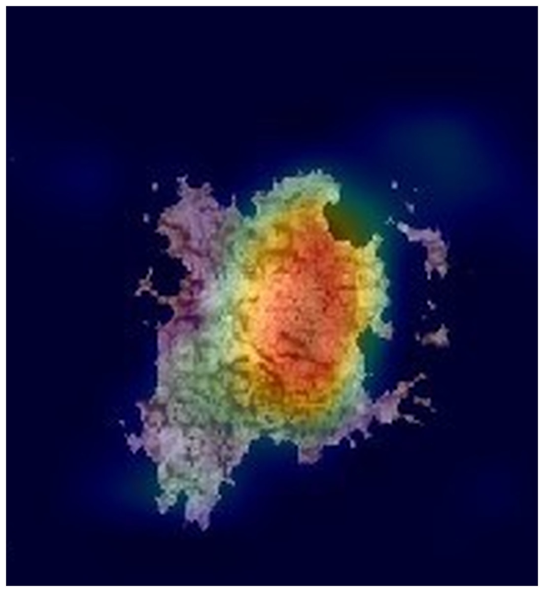
Figure 2: An example of a GRAD-CAM output extracted from the experimental dataset.
The reddest areas in the images represent the most important features for correctly classifying these images, in this case, a Melanoma.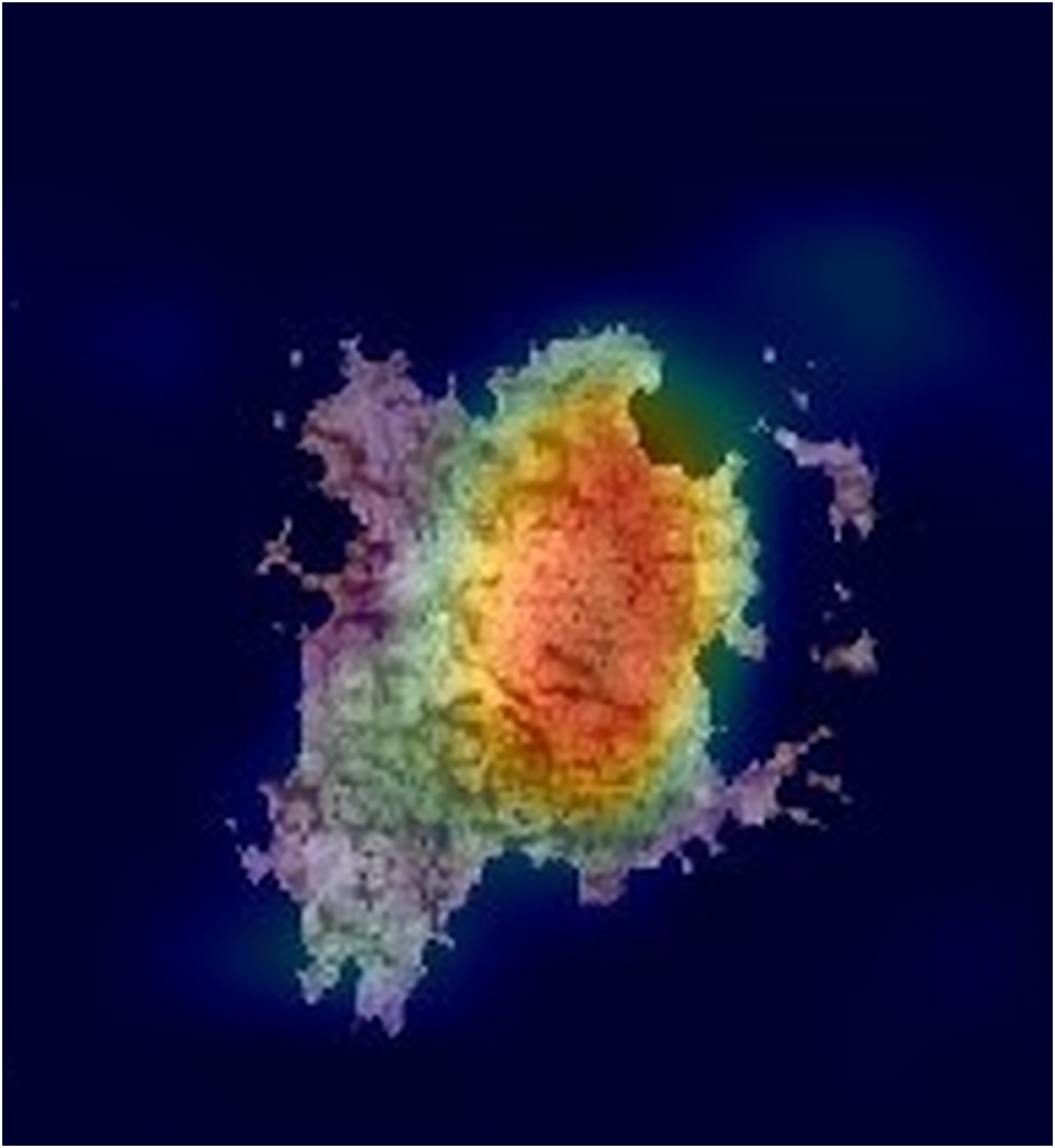
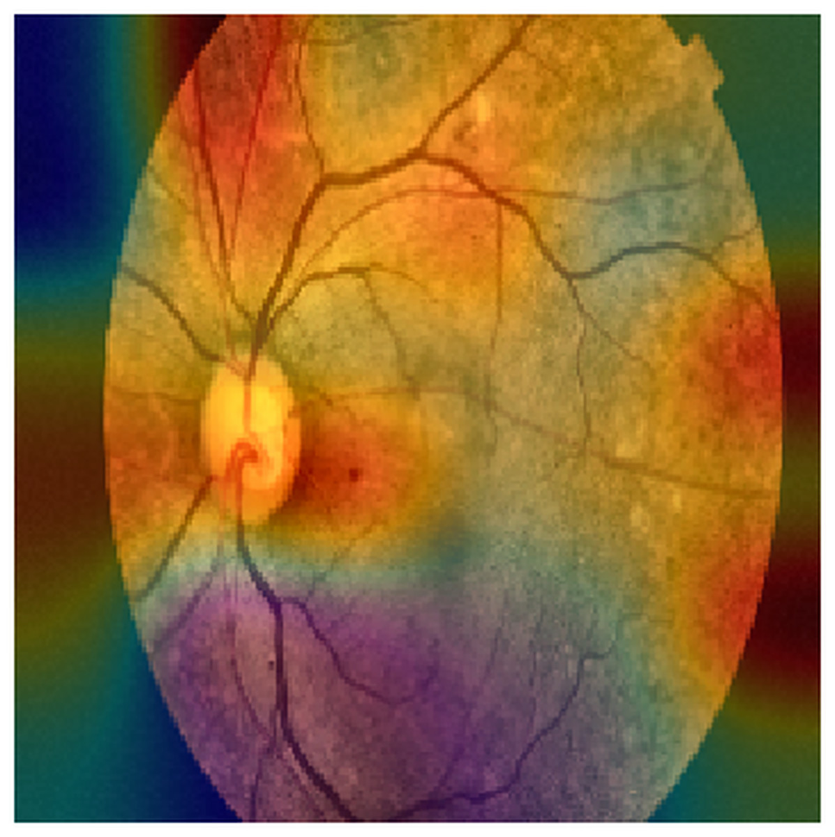
Figure 3: An example of a GRAD-CAM output extracted from the experimental dataset.
The reddest areas in the images represent the most important features for correctly classifying these images, in this case, an ocular fundus image.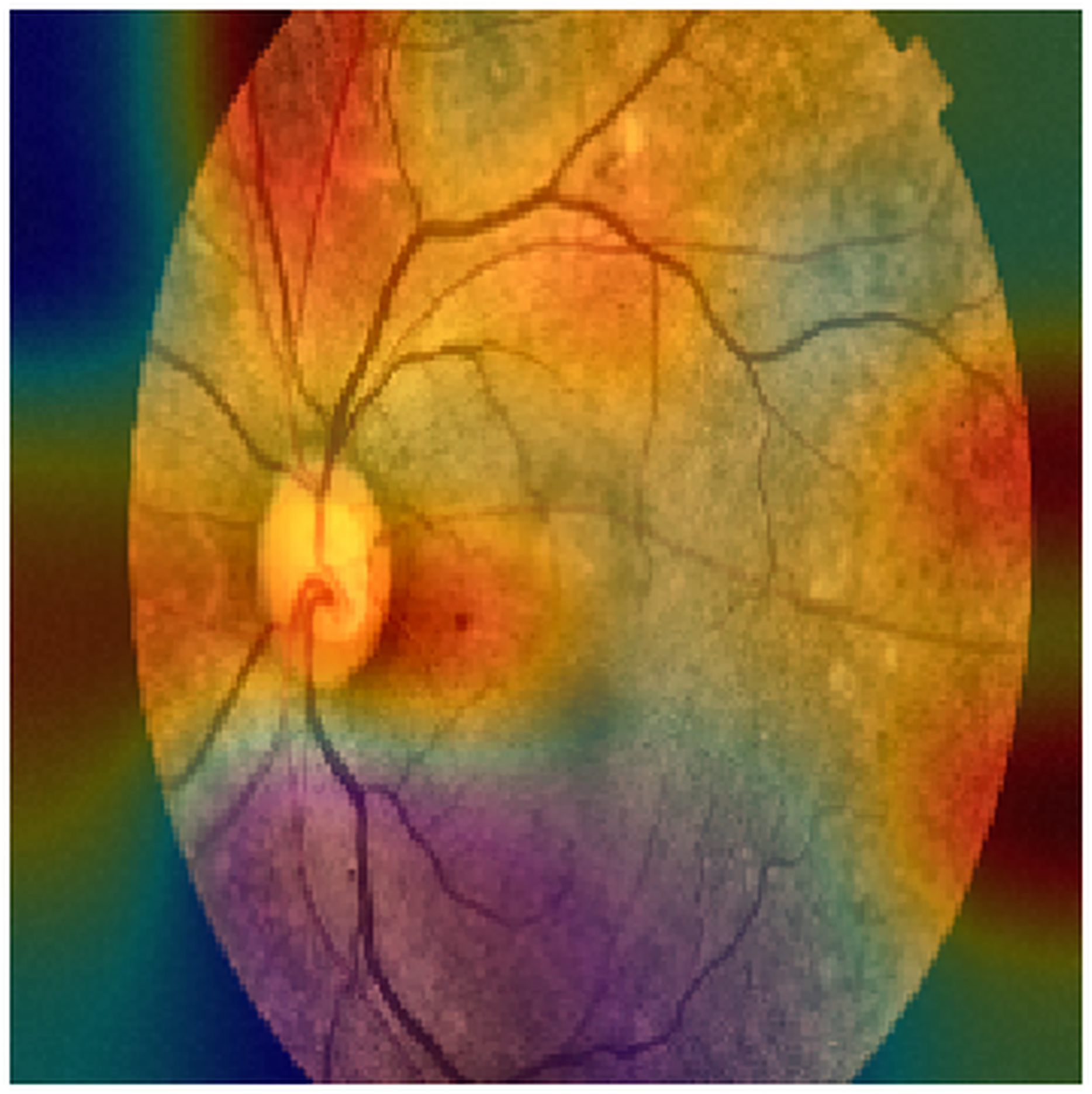
Structural similarity index measure
The Structural Similarity Index (SSIM) is a metric for evaluating the visual similarity between two images (Brunet, Vrscay & Wang, 2011). Unlike traditional pixel-based metrics like Mean Squared Error (MSE), which measure only pixel value differences, SSIM considers structural information, luminance, and contrast, providing a more perceptually relevant assessment of image quality. By comparing local patterns of pixel intensities and their spatial relationships, SSIM closely aligns with human visual perception. It outputs a value between −1 and 1, where 1 indicates perfect similarity between two images, and lower values signify perfect dissimilarity (anticorrelation). SSIM is widely used in image compression, restoration, and computer vision because it captures perceptual differences.
Performance metrics
We computed the well-established classification metrics to analyze the behavior of . We then compared with these metrics to gain insights into its strengths and weaknesses across various classification scenarios.
We report standard metrics to evaluate model performance in both binary and multiclass settings (Tables 2 and 3). For binary classification (melanoma detection), we compute Accuracy (ACC), Sensitivity (SN), Specificity (SP), Precision, and F1-score (Table 2). For multiclass classification (diabetic retinopathy grading), we compute overall Accuracy along with macro- and micro-averaged Precision, Recall, and F1-score. Macro-averaging treats each class equally, while micro-averaging reflects instance frequency. We also include Specificity, False Positive Rate (FPR), False Negative Rate (FNR), and Hamming Loss. Hamming Loss quantifies the fraction of misclassified labels, with 0 indicating perfect classification (Table 3).
| Metric | Formula |
|---|---|
| Accuracy (ACC) | |
| Sensitivity (SN) | |
| Specificity (SP) | |
| Precision (PRE) | |
| F1-score |
| Metric | Formula |
|---|---|
| Accuracy (ACC) | |
| Precision (micro) | |
| Recall (micro) | |
| F1-score (micro) | |
| Precision (macro) | |
| Recall (macro) | |
| Specificity (macro) | |
| F1-score (macro) | |
| FPR (macro) | |
| FNR (macro) | |
| Hamming loss |
Image improvements and segmentation
Due to the limited quality of the images, which are affected by poor contrast and artifacts, three different preprocessing steps were applied in this work to improve feature extraction during network training: Contrast Enhancement, Hole Erosion, and Image Segmentation. This section provides a brief introduction to these techniques.
Contrast enhancement
Enhancing contrast prior to further preprocessing or analysis improves the clarity and quality of images, making critical features more distinguishable. Contrast enhancement techniques (CE) can highlight important regions, facilitating subsequent steps such as segmentation and feature extraction (Ariateja, Ardiyanto & Soesanti, 2018). Also, CE can help improve the model’s ability to focus on relevant structures while reducing the influence of background noise.
Histogram Equalization (HE) is a classical technique that redistributes pixel intensity across the available spectrum, enhancing the overall contrast of an image. This method is beneficial in uneven lighting conditions or when the original contrast is low.
Adaptive Histogram Equalization (AHE) is a more advanced variant, which operates on small regions of the image rather than the entire image, thereby improving local contrast. However, to prevent excessive contrast amplification and the creation of artifacts, Contrast Limited Adaptive Histogram Equalization (CLAHE) is often used, introducing a limit on intensity distribution.
Another widely used technique is Gamma Correction, which modifies pixel intensity nonlinearly to emphasize darker or brighter areas of the image depending on the selected gamma value. This method is especially effective for improving image visibility with strong illumination imbalances.
Retinex-based models rely on principles of human visual perception to enhance contrast in images captured under varying lighting conditions. This technique is applied in fields such as satellite image enhancement and computer vision, as it preserves details in shadowed areas without compromising well-lit regions.
Finally, Unsharp Masking is used to increase contrast by enhancing object edges. This method involves subtracting a blurred version of the image from the original and adding the result, making details more prominent without significantly distorting the overall visual information.
Hole erosion
Hole erosion is a morphological operation to refine image data by eliminating minor artifacts, noise, or unwanted structures. This process is particularly useful in medical imaging and object detection, where fine details can interfere with classification. Hole erosion removes minor gaps and extraneous elements and improves the clarity of the main structures within the image, leading to better segmentation and analysis.
Basic erosion is one of the fundamental morphological operations. It reduces the edges of objects in the image by removing boundary pixels. While this process does not specifically eliminate “holes” in the internal regions of objects, it can be combined with other operations to refine the overall structure of the image. This technique helps remove slight noise or artifacts near object boundaries.
Morphological Closing and Opening The closing and opening operations are advanced variations of erosion used to handle holes in an image. Opening is erosion followed by dilation, which helps remove small particles and fill internal holes, while closing (followed by erosion) is effective for closing small holes. These operations are widely used to refine segmentation and enhance the quality of binary images.
Hole filling is a specific morphological technique to fill holes (empty spaces) within objects. This method “fills” missing areas without significantly altering the object’s overall shape. The algorithm analyzes the proximity of pixels and fills the holes using nearby pixels. This technique is often applied to images with disconnected objects due to artifacts or noise.
Iterative erosion involves repeatedly applying the erosion operation to an image to remove minor imperfections progressively. Each iteration removes boundary pixels that do not belong to the main object. This technique is proper when gradual noise reduction is desired or when small isolated areas within an object need to be removed.
Adaptive erosion adjusts to the local characteristics of the image. Rather than applying a fixed erosion structure, this technique uses an approach that considers intensity variations in the image. It helps improve image quality in scenarios where objects of interest vary in size or have holes of different sizes. This technique is especially helpful in complex images, where different areas must be treated differently due to noise or varying details.
Image segmentation
Image segmentation is a crucial step in preprocessing, aiming to partition an image into meaningful regions. This technique allows for the isolation of key structures relevant to classification tasks.
Thresholding is one of the simplest and most widely used segmentation techniques. It involves converting an image into a binary format by classifying pixels as either foreground or background based on their intensity values. Global thresholding applies a single threshold to the entire image, while adaptive thresholding adjusts the threshold locally for each region, which is helpful for images with varying lighting conditions.
Edge detection methods, such as the Canny or Sobel operators, are used to identify the boundaries of objects within an image. These methods highlight regions with a sharp contrast between adjacent pixels, helping to define the structure of objects. Edge detection is often followed by techniques like region growing or contour detection to complete the segmentation process.
Region-based segmentation involves dividing an image into similar regions based on specific properties such as color, texture, or intensity. Common approaches include region growing, where pixels are added to a region if they meet a predefined criterion, and region splitting and merging, where an image is recursively divided into smaller regions and then merged based on similarity.
Clustering techniques, such as k-means or mean-shift clustering, group pixels into clusters based on their feature similarity (e.g., color or texture). These methods do not require prior knowledge about the number of segments and can adapt to the structure of the image. Clustering is particularly useful when dealing with complex scenes or when the boundaries between regions are unclear.
The watershed algorithm is a region-based segmentation method that treats image intensity as topography. The image is viewed as a landscape, and regions are segmented based on the “watershed” lines where the image gradient is minimized. This method is particularly effective in separating touching or overlapping objects, and it can be used in combination with other techniques to improve accuracy.
DATASETS
EyePACS
The retinal images used in this study were obtained from EyePACS (https://eyepacs.com/). This dataset consists of a large set of high-resolution images, providing each subject’s left and right fields. The images are labelled with an ID and either ‘right’ or ‘left’ (e.g., 1_left is the left eye of patient 1). A mean then assessed the presence of diabetic retinopathy in each image using a scale from zero to four as reported in Table 4. It is important to note that this dataset may have noise in both the images and labels. Images may be out of focus, underexposed, or overexposed (https://www.kaggle.com/competitions/diabetic-retinopathy-detection/data).
| Label | Description |
|---|---|
| 0 | No DR |
| 1 | Mild |
| 2 | Moderate |
| 3 | Severe |
| 4 | Proliferative DR |
ISIC dataset
The ISIC dataset is one of the most comprehensive and well-curated collections of dermatologic images available (https://challenge.isic-archive.com/data/). It includes over 150,000 dermoscopy images linked to confirmed clinical diagnoses between 2016 and 2020. Of these, approximately 7,000 images have been made publicly accessible to the scientific community, facilitating open research and innovation in dermatology. Each image in the dataset is accompanied by detailed metadata, which provides essential context for analysis and model training. The metadata includes lesion status, classified as benign or malignant, anatomical location, and demographic information such as age and gender of the patient, which are crucial for understanding disease patterns and improving diagnostic accuracy.
Methods
The experimental analysis was conducted on two manually refined subsets of the dermatological ISIC dataset and the EyePACS dataset. A selection of state-of-the-art convolutional neural networks—excluding the Vision Transformer (ViT)—was evaluated, including AlexNet, DenseNet, EfficientNet, GoogLeNet, InceptionResNetV2, InceptionV3, MobileNetV2, ResNet18, ResNet50, ShuffleNet, VGG16, VGG19, and XCeption. Vision Transformers were not considered in this study due to several factors: (i) According to Zhu et al. (2024), CNNs are generally preferable in scenarios with limited retinal image data, as in our case and CNNs have shown superior capabilities in capturing fine-grained local features, which is particularly relevant for retinal disease tasks involving small lesions; and (ii) hardware constraints further limited the feasibility of training ViT-based models. Nonetheless, future work should investigate the robustness of the proposed indicator for Vision Transformer architectures, potentially exploring hybrid solutions that integrate CNNs with ViTs.
The proposed framework implementation is available at https://doi.org/10.5281/zenodo.15553645.
Also, for full implementation details and step-by-step instructions for dataset preparation, model training, evaluation, and trustworthiness computation, please refer to the included README file available at: https://github.com/CAISLab-Unisa/trustworthiness/blob/main/README.md.
Selection method
The selection of the techniques implemented in this work was guided by their relevance to the medical image classification tasks addressed, their support for model interpretability, and their potential to contribute to the assessment of trustworthiness in AI-based diagnostic systems.
CNN were chosen as the primary models due to their established effectiveness in tasks such as melanoma detection and DR grading. A diverse set of architectures was included, ranging from lightweight to deeper models, to capture a broad spectrum of learning behaviors and assess the consistency of internal feature representations across different network types.
Grad-CAM was selected as the interpretability method because it enables the visualization of class-discriminative regions in input images, allowing clinicians to inspect and validate the reasoning behind model predictions. This choice aligns with the growing demand for explainability in AI applications within the healthcare sector.
The Trustworthiness Indicator proposed in this study was specifically designed to measure the consistency of activation patterns across models based on the hypothesis that high agreement among independently trained models may signal robust and generalizable decision processes.
The selection of public datasets—ISIC for skin lesion classification and EyePACS for retinal disease grading—was driven by their clinical relevance, size, and widespread use in benchmarking AI models, ensuring that the evaluation would be grounded in real-world scenarios.
Computing infrastructure
The experiments were conducted on a workstation running Windows 11 version 24H2 (build 26100.4061), equipped with an AMD Ryzen Threadripper PRO 5955WX 16-core processor (32 threads, 4 GHz), 128 GB of RAM, and a single NVIDIA RTX A4000 GPU with 16 GB of VRAM. The implementation was developed using MATLAB R2023b with the Parallel Computing Toolbox and Deep Learning Toolbox.
Image pre-processing
For the ISIC dataset, we use a Sobel-based edge segmentation pipeline combined with morphological refinements. We first applied k-means clustering with two clusters, followed by hole filling. We converted the image to grayscale, and an automatic Sobel threshold was computed; this value was then scaled by a fudge factor of 0.5 to obtain a more conservative edge map. To connect fragmented edges, we applied dilation with linear structuring elements of size 5 (90∘) and 3 (0∘). Subsequently, residual holes were filled, border-touching artifacts were removed using 4-connectivity, and two successive erosions with a diamond structuring element of radius 2 were performed. The final mask was applied to the original image to isolate the region of interest. No watershed transform was employed in this workflow.
For the EyePACS dataset, we enhanced image contrast in the luminance channel using Contrast Limited Adaptive Histogram Equalization (CLAHE). Images were converted to the CIE-Lab color space, the L channel was normalized, processed with adapthisteq using MATLAB default parameters, and then reconverted to RGB. This approach enhanced the visibility of relevant structures while minimizing the amplification of noise. No additional denoising, class rebalancing, or label-noise handling was applied at this stage, as the aim of the study was not to optimize predictive accuracy but rather to evaluate the behavior of the proposed reliability indicator under realistic conditions.
For reproducibility, the exact MATLAB scripts used for these steps are made available in the project repository.
Network preparation
To prepare the networks, a specific configuration of the AlexNet architecture was designed for training from scratch. In this version, the network is initialized without pre-trained weights, so all parameters start from random values, and the entire model is trained from the beginning. The input layer is adapted to match the specified INPUT_SIZE, ensuring compatibility with the input data. The final fully connected layer (fc8) is replaced to produce many outputs equal to OUTPUT_CLASSES, corresponding to the number of target classes in the classification task (2 for melanoma and 5 for DR).
Training setup
In our experimentation, two distinct training configurations were established to evaluate the impact of data augmentation on the performance of a neural network. The first configuration involved standard training without any augmentation, while the second introduced various random transformations to the training images aimed at increasing dataset diversity and enhancing the model’s ability to generalize. Data augmentation techniques included random horizontal reflections simulating mirrored images to introduce orientation variability. In addition, random translations were applied along the horizontal and vertical axes, allowing shifts within a range of −180 to 180 pixels. Images were randomly scaled in both dimensions, with scaling factors sampled between 1 and 30. These transformations were selected to mimic a broad spectrum of real-world variations in object positioning, size, and orientation, thereby increasing the robustness of the model.
Both configurations employed the same optimization strategy, based on stochastic gradient descent with momentum (SGDM), using an initial learning rate of 0.0001, a maximum of 20 training epochs, and mini-batches of 50 samples. The dataset was shuffled during training at the beginning of each epoch, and validation was performed every 100 iterations. The training process was monitored through real-time visual feedback, while intermediate textual outputs were suppressed. In order to ensure computational efficiency, training was executed using GPU acceleration; however, the experimentation is reproducible using CPUs. The only difference between the two setups lies in the validation dataset: the first configuration used the original, unaugmented validation set, while the second employed an augmented version of the validation data, incorporating the same transformation strategies used during training. This controlled setup directly compares model performance under conditions with and without data augmentation.
Training starts by selecting the training dataset from a predefined split, in which the entire dataset has been partitioned into training, validation, and test sets according to a specified ratio. A string identifier representing the split configuration was generated and used to organize the results of each experiment. This identifier dynamically created a structured directory hierarchy to store outputs, including the dataset name, model name, and split configuration: this choice ensured that all experiment results were stored in uniquely identifiable and reproducible locations. The model was then trained using the designated architecture, the selected training data, and the defined training parameters.
Performance evaluation and logging
The resulting model and its performance metrics were saved, including a graphical representation of the training progress, enabling post-hoc analysis of learning dynamics. The evaluation phase continued on the test set, where the model’s classification performance was quantitatively assessed. In addition, visual interpretability techniques—specifically Grad-CAM—were applied to generate saliency maps that highlight the regions of input images most influential in the model’s predictions. All results were systematically stored in a structured directory, organized by dataset and model identifiers, and computations were performed using GPU acceleration where applicable.
In order to evaluate the model’s generalization capabilities, a standardized procedure was followed to test performance on all three dataset partitions: training, validation, and testing. The evaluation process involved classifying each partition and comparing the predicted labels to the corresponding ground truth. The classification accuracy for each set was computed and logged, along with relevant metadata such as the dataset name, the network configuration, and the data split ratios used during training. Results were saved in a tab-separated values file to facilitate subsequent analysis.
In addition to accuracy metrics, confusion matrices were generated for each data partition to provide a more detailed view of classification performance across individual classes. These matrices were saved in plain text format, and corresponding visual charts were exported as image files. The evaluation pipeline was designed for repeatability and transparency, ensuring that each experiment produced a complete and traceable set of outputs within a clearly defined directory structure.
Gradcam extraction and handling
Grad-CAM generates visual explanations of network predictions by producing heatmaps highlighting image regions most influential to the model’s decisions. In our setup, this process takes the dataset name, network name, data split configuration, and test set as input, establishing a structured directory layout based on these parameters and the predicted class labels. Each result consists of a heatmap, produced using the gradCAM function, superimposed on the original image to form an interpretable visualization. These composite images are saved in class-specific folders in .png format to facilitate visual inspection, automatic similarity structure analysis, and comparative evaluation across test samples.
To formalize this step, we denote as the -th image in the test set TS, and as the -th network in the set of trained-from-scratch models TNN. The scoreMap, as defined in (https://it.mathworks.com/help/deeplearning/ref/gradcam.html), encodes regions with high activation values that contributed most to the prediction made by . For each and , we compute the pair , where is the scoreMap, and is the resulting composite image obtained by overlaying on using the jet colormap (https://it.mathworks.com/help/matlab/ref/jet.html).
Trustworthiness definition
In order to link how differently each network uses different features to make choices with our WH, we defined a Pair Consensus Indicator ( ). In this work, and a value near 1 indicates max consensus.
Specifically, we used a composition of the function that integrates the SSIM to compute the similarity between two generic images, as explained in the equation below (Eq. (2)).
(1)
(2)
SSIM takes values between −1 and 1, with 1 indicating max correlation and −1 max anti-correlation. Therefore, takes value on .
If we consider two generic neural network models that work with images, and , and an image , we can define:
(3) as the correlation-distance between activation features used by network and to choose an answer (the class predicted) and , regarding the image . In the formula, and denote the Grad-CAM score maps for and on image .
Therefore, is the prediction of regarding image . This correlation distance is what we define as consensus on feature selections between two different NN models. As a result of the corrected ssim property, takes on a positive and increasing value the higher the correlation between activation features is, and therefore, the higher the consensus between feature choices.
However, at this point, it is important to note that activation pattern similarity does not necessarily directly correlate with trustworthiness. NN can share activations even when making incorrect predictions, particularly in overfitted models. It is mandatory to consider that a high value of only indicates a high consensus about features used to make a decision (networks use similar features to make a prediction). Therefore, we have to take into account wrong decisions.
If denotes the ground-truth class for image , and and are the labels predicted by and , respectively, we define the choice-level network consensus as follows.
Choice-level network consensus and label mapping. Let denote the softmax probability vector predicted by network for image . The corresponding predicted label is
(4)
An analogous definition holds for with . In the binary case ( ), this is equivalent to thresholding the positive-class probability (or logit) at . We denote by the ground-truth class of image .
Let be the ground-truth class of image , and let and be the labels predicted by networks and , respectively. We define the choice-level network consensus as
(5)
Therefore, given a dataset composed of images and two NN and , we can compute what we defines as Local Trustworthiness of a network pair against D as follow:
(6)
Due to the presence of the penalty in , please note that take values in [−1, 1].
If we consider a set of and P(TNN) as the set of all possible pairs within TNN, we can generalize in Trustworthiness of a CNN set against the classification problem on D as follow:
(7)
Also, as defined, it is possible to compute against a specific prediction class (for example, benign or melanoma or severe or mild retinopathy).
In that case, the dataset comprises images of the same class , defined as .
(8)
Results
Table 5 summarizes the classification performance of CNN models trained from scratch. In the melanoma scenario, all networks achieved satisfactory accuracy, with notable results from: ResNet50, which achieved a recall of 95.50% and F1-score of 84.80%, though its specificity was moderate (63.74%); GoogleNet, with a more balanced performance: recall of 85.59%, specificity of 78.02%, and F1-score of 84.07%. In the diabetic retinopathy task, VGG19 yielded the best overall performance, with accuracy, precision, recall, and F1-score all above 93%. VGG16 followed closely with an accuracy of 86.63% and a macro recall of 71.59%. These results confirm that CNNs can perform reliably in image-based medical classification tasks, with some architectures outperforming others depending on the specific problem and class distribution.
| Melanoma detection | Diabetic retinopathy graduation | ||||||||||||
|---|---|---|---|---|---|---|---|---|---|---|---|---|---|
| Model | ACC (%) | Precision (%) | Recall (%) | Specificity (%) | F1-score (%) | FPR (%) | FNR (%) | ACC (%) | SN (%) | SP (%) | PRE (%) | F1 (%) | FPR (%) |
| AlexNet | 80.20% | 75.18% | 95.50% | 61.54% | 84.13% | 38.46% | 4.50% | 84.86% | 84.86% | 95.60% | 84.86% | 84.86% | 4.40% |
| DenseNet | 80.20% | 75.18% | 95.50% | 61.54% | 84.13% | 38.46% | 4.50% | 75.17% | 75.17% | 93.42% | 75.17% | 75.17% | 6.58% |
| EfficientNet | 81.19% | 78.29% | 90.99% | 69.23% | 84.17% | 30.77% | 9.01% | 81.58% | 81.58% | 95.09% | 81.58% | 81.58% | 4.91% |
| GoogleNet | 82.18% | 82.61% | 85.59% | 78.02% | 84.07% | 21.98% | 14.41% | 76.26% | 76.26% | 93.25% | 76.26% | 76.26% | 6.75% |
| InceptionResNetV2 | 81.19% | 77.86% | 91.89% | 68.13% | 84.30% | 31.87% | 8.11% | 78.85% | 78.85% | 94.00% | 78.85% | 78.85% | 6.00% |
| InceptionV3 | 77.72% | 73.24% | 93.69% | 58.24% | 82.21% | 41.76% | 6.31% | 79.13% | 79.13% | 94.33% | 79.13% | 79.13% | 5.67% |
| MobileNetV2 | 78.71% | 76.56% | 88.29% | 67.03% | 82.01% | 32.97% | 11.71% | 70.80% | 70.80% | 92.28% | 70.80% | 70.80% | 7.72% |
| ResNet18 | 80.20% | 76.69% | 91.89% | 65.93% | 83.61% | 34.07% | 8.11% | 76.94% | 76.94% | 93.45% | 76.94% | 76.94% | 6.55% |
| ResNet50 | 81.19% | 76.26% | 95.50% | 63.74% | 84.80% | 36.26% | 4.50% | 75.44% | 75.44% | 93.46% | 75.44% | 75.44% | 6.54% |
| ShuffleNet | 80.20% | 76.30% | 92.79% | 64.84% | 83.74% | 35.16% | 7.21% | 74.62% | 74.62% | 92.76% | 74.62% | 74.62% | 7.24% |
| VGG16 | 80.69% | 80.00% | 86.49% | 73.63% | 83.12% | 26.37% | 13.51% | 86.63% | 86.63% | 96.36% | 86.63% | 86.63% | 3.64% |
| VGG19 | 78.81% | 83.78% | 83.78% | 72.53% | 81.22% | 27.47% | 16.22% | 93.19% | 93.19% | 98.13% | 93.19% | 93.19% | 1.87% |
| XCeption | 77.33% | 76.09% | 94.59% | 45.90% | 84.34% | 54.10% | 5.41% | 72.44% | 72.44% | 92.40% | 72.44% | 72.44% | 7.60% |
Although Table 5 reports standard performance metrics that are not themselves measures of explainability, they serve as a baseline for interpreting the trustworthiness values in Tables 6 and 7.
| AlexNet | DenseNet | EffNetB0 | GoogleNet | IncResNetV2 | InceptionV3 | MobileNetV2 | ResNet18 | ResNet50 | ShuffleNet | VGG16 | VGG19 | XCeption | |
|---|---|---|---|---|---|---|---|---|---|---|---|---|---|
| AlexNet | 0.96 | 0.22 | 0.15 | 0.21 | 0.22 | 0.24 | 0.09 | 0.14 | 0.14 | 0.19 | 0.07 | 0.11 | 0.19 |
| DenseNet | 0.96 | 0.19 | 0.05 | 0.37 | 0.27 | 0.22 | 0.35 | 0.38 | 0.26 | 0.19 | 0.11 | 0.44 | |
| EffNetB0 | 0.91 | −0.01 | 0.17 | 0.09 | 0.09 | 0.07 | 0.12 | 0.27 | 0.29 | 0.46 | 0.12 | ||
| GoogleNet | 0.86 | −0.01 | 0.27 | −0.04 | −0.02 | −0.03 | 0.05 | −0.06 | 0.04 | −0.01 | |||
| IncResNetV2 | 0.92 | 0.20 | 0.24 | 0.32 | 0.36 | 0.26 | 0.18 | 0.10 | 0.43 | ||||
| InceptionV3 | 0.94 | 0.12 | 0.14 | 0.15 | 0.23 | 0.07 | 0.07 | 0.20 | |||||
| MobileNetV2 | 0.88 | 0.25 | 0.26 | 0.17 | 0.15 | 0.03 | 0.27 | ||||||
| ResNet18 | 0.92 | 0.53 | 0.16 | 0.14 | 0.02 | 0.47 | |||||||
| ResNet50 | 0.96 | 0.22 | 0.16 | 0.03 | 0.47 | ||||||||
| ShuffleNet | 0.93 | 0.19 | 0.19 | 0.22 | |||||||||
| VGG16 | 0.87 | 0.29 | 0.18 | ||||||||||
| VGG19 | 0.84 | 0.06 | |||||||||||
| XCeption | 0.95 |
| AlexNet | DenseNet | EffNetB0 | GoogleNet | IncResNetV2 | InceptionV3 | MobileNetV2 | ResNet18 | ResNet50 | ShuffleNet | VGG16 | VGG19 | XCeption | |
|---|---|---|---|---|---|---|---|---|---|---|---|---|---|
| AlexNet | 0.62 | −0.05 | −0.10 | −0.04 | −0.04 | −0.11 | −0.07 | −0.03 | −0.04 | −0.06 | −0.05 | −0.06 | −0.09 |
| DenseNet | 0.62 | 0.06 | −0.14 | 0.05 | −0.05 | 0.02 | 0.03 | 0.03 | −0.03 | 0.16 | 0.11 | 0.08 | |
| EffNetB0 | 0.69 | −0.15 | 0.06 | −0.08 | 0.04 | 0.03 | 0.02 | 0.09 | 0.22 | 0.25 | 0.01 | ||
| GoogleNet | 0.78 | −0.10 | −0.07 | −0.10 | −0.10 | −0.13 | −0.16 | −0.08 | −0.09 | −0.15 | |||
| IncResNetV2 | 0.68 | −0.01 | 0.08 | 0.12 | 0.07 | 0.07 | 0.15 | 0.15 | 0.17 | ||||
| InceptionV3 | 0.58 | −0.09 | −0.03 | −0.03 | −0.07 | −0.01 | −0.03 | −0.04 | |||||
| MobileNetV2 | 0.67 | 0.05 | 0.01 | 0.01 | 0.08 | 0.05 | 0.03 | ||||||
| ResNet18 | 0.66 | 0.18 | 0.06 | 0.10 | 0.09 | 0.10 | |||||||
| ResNet50 | 0.64 | 0.02 | 0.08 | 0.07 | 0.04 | ||||||||
| ShuffleNet | 0.65 | 0.10 | 0.12 | −0.01 | |||||||||
| VGG16 | 0.74 | 0.35 | 0.12 | ||||||||||
| VGG19 | 0.73 | 0.11 | |||||||||||
| XCeption | 0.64 |
Table 3 further complements this analysis by reporting DR-specific metrics, which, when considered together with , illustrate how the indicator provides information beyond accuracy.
The proposed trustworthiness indicator , based on the internal activation similarity among CNNs, was evaluated on a per-class basis. Tables 6 and 7 report the pairwise values for the benign and malignant melanoma classes, respectively. Note that the diagonal entries are below 1.00 because each architecture was trained independently; thus, even networks with the same design exhibit variability in their internal activations and therefore in consensus. Only a network compared with itself (identical weights) would yield .
The results show significant variability in the internal activation pattern consistency among model pairs: High values (e.g., AlexNet–DenseNet = 0.96 for benign class) indicate strong agreement in internal features used for predictions. Low or even negative values (e.g., GoogleNet–ShuffleNet = −0.16 for malignant class) suggest divergence in feature selection, even when prediction accuracy remains high: this confirms that CNNs with similar accuracy may rely on different internal representations. Therefore, classical metrics such as accuracy or F1-score do not necessarily reflect model robustness or consensus.
From a comparative perspective, the trustworthiness indicator offers complementary insights beyond those captured by traditional classification metrics such as accuracy, precision, recall, and F1-score. While classical metrics evaluate model performance based solely on prediction correctness, focuses on the internal consistency of feature activations across different neural architectures. Additional macro-level metrics for diabetic retinopathy grading are reported in Table 8, further supporting the comparative analysis of model performance.
| Model | SN macro (%) | PRE macro (%) | F1 macro (%) | FPR macro (%) | FNR macro (%) | HALO (%) |
|---|---|---|---|---|---|---|
| AlexNet | 70.56% | 79.46% | 73.85% | 4.40% | 29.44% | 15.14% |
| DenseNet | 53.24% | 55.00% | 53.97% | 6.58% | 46.76% | 24.83% |
| EfficientNet | 63.66% | 70.15% | 65.99% | 4.91% | 36.34% | 18.42% |
| GoogleNet | 53.50% | 63.66% | 54.44% | 6.75% | 46.50% | 23.74% |
| InceptionResNetV2 | 56.92% | 67.37% | 57.92% | 6.00% | 43.08% | 21.15% |
| Inception V3 | 60.22% | 65.03% | 61.99% | 5.67% | 39.78% | 20.87% |
| MobileNetV2 | 45.52% | 46.44% | 45.74% | 7.72% | 54.48% | 29.20% |
| ResNet18 | 55.19% | 61.69% | 57.08% | 6.55% | 44.81% | 23.06% |
| ResNet50 | 51.90% | 54.02% | 52.40% | 6.54% | 48.10% | 24.56% |
| ShuffleNet | 47.63% | 57.15% | 47.87% | 7.24% | 52.37% | 25.38% |
| VGG16 | 71.59% | 80.35% | 74.63% | 3.64% | 28.41% | 13.37% |
| VGG19 | 87.10% | 90.65% | 88.75% | 1.87% | 12.90% | 6.82% |
| XCeption | 49.31% | 51.60% | 50.14% | 7.60% | 50.69% | 27.56% |
Experiments reveal that high predictive performance does not always correlate with high values. For instance, some models such as XCeption and InceptionV3 achieved competitive F1-scores but showed lower values in pairwise comparisons, indicating less agreement in the internal reasoning process. Conversely, models like AlexNet and DenseNet exhibited high values (e.g., 0.96 for benign class) despite not always leading in terms of accuracy or recall: this suggests that may capture an orthogonal property of model behavior—specifically, the robustness and generalizability of feature representations.
Correlation between the trustworthiness indicator Φ and classical performance metrics
We investigated whether a statistical relationship exists between and classical performance indicators. Preliminary correlation analyses suggest that the relationship between and metrics such as accuracy, precision, and F1-score is weak or nonlinear. In some cases, local positive trends can be observed—e.g., moderate values tend to co-occur with balanced precision and recall, but these trends break down when outlier architectures (e.g., those with overfitting or underfitting behavior) are included.
To assess the statistical relationship between and traditional performance indicators, we first computed for each network the mean pairwise trustworthiness on the malignant melanoma class:
where are the values reported in Tables 6 and 7. We then assembled vectors of classical metrics, for example
using the results in Table 5.
Pearson’s correlation coefficient and Spearman’s rank correlation were then computed between and each performance vector. In all cases, and , corresponding to for every linear regression. Further, standard transformations (logit, arcsine of proportions, and second-order polynomial fits) did not increase the best above 0.10. These results indicate that captures an internal model-agreement dimension largely orthogonal to classical accuracy-based metrics.
Given the bounded nature of , and the inherently bounded classical metrics , we also considered whether the relationship could be linearized through transformations such as logit, arcsin, or polynomial regression. However, even under these transformations, the overall coefficient of determination ( ) remained low across all tests: this reinforces the hypothesis that and classical metrics capture distinct dimensions of model evaluation.
Notably, the malignant class consistently exhibits lower and more variable values across all model pairs: this may reflect the inherent ambiguity or variability in pathological patterns associated with malignant melanoma, leading to divergent internal representations even among well-performing classifiers. Such discrepancies could be clinically significant, indicating reduced model consensus in high-risk cases.
The statement regarding the bounded nature of and the failure of standard linearizing transforms is grounded in our quantitative correlation experiments. We first extracted each network’s mean pairwise trustworthiness on the malignant melanoma class:
Using the values in the trust matrix (Table 6 for benign and the corresponding matrix for malignant). Classical performance vectors, for example
were taken directly from Table 5 Computing Pearson’s and Spearman’s between and each metric yielded , , and for all linear fits. We then applied logit, arcsin transforms, and second-order polynomial regression, but the best remained below 0.10: this demonstrates that resides in and classical metrics in , yet no simple transform produces a strong linear relationship—hence our conclusion that the two capture distinct evaluation dimensions.
The observation that the malignant class exhibits more dispersed values follows from summary statistics on the pairwise entries. If we denote as all network pairs, we compute for each class :
For the malignant melanoma class, we found , , whereas for the benign class , .
The larger standard deviation and the broader range of values in the malignant class reflect greater model disagreement in high-risk cases, underscoring potential clinical significance when consensus among classifiers is low.
Discussion, conclusions and future work
This work introduces a Trustworthiness Indicator designed to quantify the reliability of CNN-based models through internal activation pattern consistency, applied to classifying melanoma and diabetic retinopathy (DR). The formulation of integrates the similarity of Grad-CAM-derived activation maps and the predictive agreement across neural network pairs, offering a different perspective than classical performance metrics.
Regarding the first research question (RQ1), the indicator appears capable of capturing structural coherence in model decision-making. In the case of melanoma classification, specific network pairs exhibited high similarity in activation maps and prediction outcomes. However, this coherence was inconsistent across all pairs, and even high-performing models such as AlexNet and ResNet50 demonstrated different activation behaviors.
Figure 4 illustrates that networks can achieve comparable accuracy while relying on divergent feature representations. This variability indicates that accuracy alone cannot ensure clinical reliability. highlights when high-performing models diverge in their internal reasoning by explicitly quantifying the stability of activation patterns, and provides insight into robustness and interpretability beyond predictive accuracy. The divergence is even more evident in the DR scenario, where the complexity and variability of retinal images contribute to larger fluctuations in the trustworthiness values. These results suggest that can serve as a complementary tool to identify models that are not only accurate but also consistent and reliable, particularly in data-limited or high-noise scenarios.
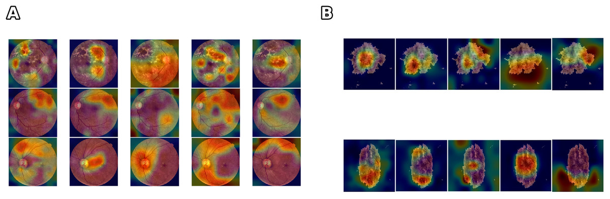
Figure 4: Comparison of feature learning across different networks for skin lesion and class differentiation.
(A) Five different networks learn very different features from the same benign and malignant skin lesions (one lesion per row) but still achieve high accuracy, (B) Five different networks learn very different features from the same mild, severe, and healthy classes (one class per row) but still achieve high accuracy.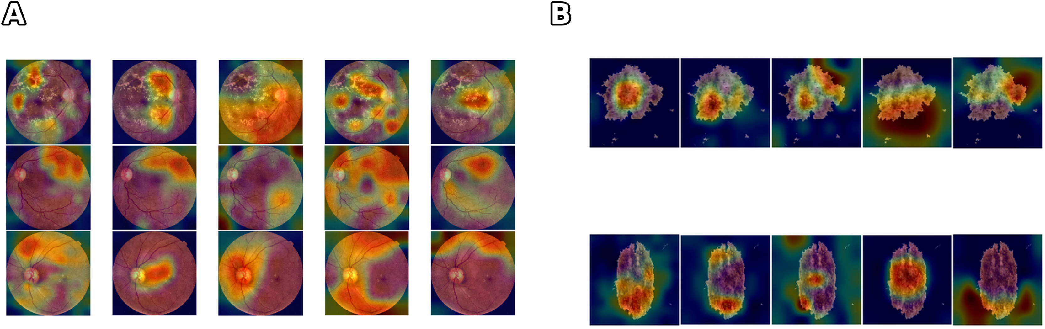
Concerning the second research question (RQ2), the analysis confirms that combining models does not guarantee increased trustworthiness. Ensemble systems may improve classical metrics such as accuracy or recall, but the overall value may remain low or even degrade without aligned internal representations. This is observed in cases where models with high individual performance fail to produce convergent activation maps when jointly analyzed. Consequently, the absence of shared internal structures suggests that ensemble methods must be carefully designed, prioritizing both output diversity and consistency in feature extraction.
It is essential to clarify how the proposed indicator differs from and complements existing XAI metrics such as SHAP or LIME.
Whereas SHAP and LIME provide local post-hoc explanations of individual predictions by attributing importance to specific features, captures the internal consistency of models by comparing activation patterns and prediction agreement across networks. In this sense, does not replace interpretability methods but complements them: while saliency or attribution maps explain why a model makes a specific decision, quantifies how consistently different models rely on similar internal representations.
This dual perspective is particularly relevant in clinical contexts, where both interpretability (explanation of a decision) and reliability (consistency of reasoning) are necessary to establish trust in AI-assisted diagnosis.
Limitations
The EyePACS dataset is known to contain noisy labels due to inter-observer variability in grading. The ISIC dataset presents class imbalance, with fewer melanoma cases compared to benign lesions. While we did not apply additional strategies to address these issues, this choice aligns with the focus of our study, which was to evaluate the reliability indicator rather than to maximize predictive accuracy.
A further limitation of this study is that we restricted our analysis to CNN-based architectures. Although EfficientNet and Vision Transformers represent more recent models, their inclusion was beyond the scope of this work due to computational constraints (EfficientNet) and the need for different interpretability approaches (e.g., attention rollout for transformers) that are incompatible with our framework. Future work should extend the proposed reliability indicator to these architectures to evaluate its robustness across diverse model families.
Other main limitations of the current formulation lies in the definition of the similarity function , which is constrained to the range by the application of a rectified version of SSIM. In particular, the current formulation:
(9)
This truncation ensures interpretability of but may also reduce the sensitivity of to strong divergences, since all negative SSIM values are treated equally as zero, but it does not fully exploit the information provided by anti-correlated activations since negative SSIM values are nullified.
A refined formulation could preserve this information, potentially leading to a more nuanced characterization of divergence in feature selection. A sensitivity analysis, or the use of alternative similarity measures that preserve anti-correlation information, will be essential to assess the practical impact of this design choice.
Additionally, the current indicator penalizes disagreement but does not reward positive consensus. The definition of could be generalized to account for premiality by introducing weighted constants P and L as follows:
(10)
P represents a reward for correct joint classification and L a penalty otherwise. This formulation would allow to reflect the level of agreement in predictions and their correctness.
Our current definition of is label-based and does not distinguish between low-confidence agreement (e.g., ) and high-confidence agreement (e.g., ). A straightforward extension is to weight by model confidence. In the generalized form
(11) one can set
(12) where and are the softmax probability vectors predicted by networks and , respectively. As an alternative fully probabilistic variant that maps to without hard thresholding, one may define
(13) which increases only when both networks assign high probability to the correct class.
Another important point concerns the robustness of the indicator. Since is computed over a specific train-validation-test split, it reflects the trustworthiness of a model set under particular data partitioning. Future work should investigate the stability of across multiple splits to assess whether the indicator generalizes or is sensitive to data shuffling. This aspect is relevant to evaluating whether trustworthiness is an intrinsic model property or an artifact of the experimental design.
From a methodological standpoint, it is worth noting that a distance-like function could be defined using an inverted similarity operator:
(14) and thus
(15)
In this context, measures dissimilarity rather than similarity, and would equal zero if and only if the two networks are perfectly correlated. Investigating whether satisfies the triangle inequality and other properties typical of a metric could open up a path toward formalizing within a proper mathematical framework.
The formulation of assumes that agreement in internal representations is a proxy for trustworthiness. However, this assumption requires further experimental validation, possibly including human-in-the-loop settings or reinforcement schemes where influences model updating based on expert feedback. Such integration would move toward a symbiotic AI paradigm in which interpretability and performance co-evolve, guided by algorithmic and human criteria.
An important limitation of the current work is the absence of probabilistic calibration analysis, specifically the lack of integration with metrics such as the Expected Calibration Error (ECE). While the indicator measures internal consistency among CNNs, it does not consider the alignment between predicted probabilities and empirical frequencies. A model can achieve high accuracy and even high values while remaining poorly calibrated, potentially overestimating or underestimating risk by large margins: this is particularly critical in clinical applications, where predicted probabilities often guide threshold-based interventions. Recent studies have also shown that models optimized for fairness may sacrifice calibration performance, revealing inherent trade-offs in multi-objective optimization. As a result, future developments of the trustworthiness framework should explore the combination of with probabilistic calibration metrics to ensure both interpretability and actionable reliability in AI-assisted diagnosis.
Conclusion and future work
In conclusion, the proposed indicator represents a first step toward quantifying internal trust in AI systems, especially in healthcare, where decisions must be accurate but also transparent and dependable. While the initial results are promising, much work remains to formalize and validate in diverse clinical contexts.
Future work will involve validating the proposed reliability indicator across a broader range of clinical domains and datasets, as well as exploring its integration with emerging architectures such as transformers and hybrid radiomics–deep learning models. Additionally, user studies with clinicians could provide valuable insights into the practical applicability and trustworthiness of the indicator in real-world healthcare settings. Also, future studies may incorporate noise-robust training methods for EyePACS and class-balancing techniques for ISIC to examine whether the reliability indicator maintains its validity when model performance is further optimized.
Reproducibility and implementation details
To ensure the full reproducibility of our experiments, we provide implementation and execution instructions in a public repository (https://github.com/CAISLab-Unisa/trustworthiness). The immutable snapshot related to the source code for this contribution is available on ZENODO: https://doi.org/10.5281/zenodo.15553645.
Below is a summary of the essential components.
Requirements
MATLAB R2023b, Deep Learning Toolbox, and a GPU with at least 12GB VRAM are recommended. The pipeline is also compatible with only CPU devices. However, the running time will be higher.
Datasets
We use the ISIC skin lesion dataset (Rotemberg et al., 2021) and the EyePAC dataset (Cuadros & Bresnick, 2009). Both datasets are public. To download the correct ISIC images for reproducing our experiment, please refer to the file ISIC_Image_Labels.txt provided in the repository. The full link to download datasets are reported in the previous sections (see footnotes).
Preprocessing
Scripts for image enhancement (histogram equalization, contrast adjustment, hole erosion) are included: otsu_he.m for ISIC and rgb9cer_improve.m for EyePAC.
Model training
The training pipeline is implemented in Step1_Run_CNN_Trainings.mlx, supporting 19 CNN architectures trained from scratch. Please note that the pipeline is also capable of performing experimentation using fine-tuning and transfer learning, but for the scope of this contribution, these features must remain deactivated to reproduce this experimentation. The provided code is configured to reproduce this experimentation.
Usage instructions
These steps must be performed to ensure reproducibility. In each script, Set rng(0) and rand(0). The provided scripts are pre-configured with these parameters.
To switch between Melanoma and RD experimentation, you need to adjust the dataset path, number of output classes, and experiment name, as specified in the provided code and README. Md file explains how to perform this action. Please note that results (trained models, metrics, confusion matrices) are saved in a structured folder hierarchy.
Trustworthiness computation
Scripts Step2_Generate_Phi_By_Pairs.mlx and Step3_Generate_CNN_Pairs_Labels_Predictions.mlx compute Grad-CAM similarity and prediction consensus. Final values can be computed via pre-configured Excel sheets in the repository.