Crossfire: cross-domain feature integration for robust time series classification
- Published
- Accepted
- Received
- Academic Editor
- Feng Gu
- Subject Areas
- Artificial Intelligence, Data Mining and Machine Learning, Data Science, Optimization Theory and Computation, Scientific Computing and Simulation
- Keywords
- Time series classification, Time series features, Feature engineering, Transformations, Efficiency
- Copyright
- © 2025 Alagöz
- Licence
- This is an open access article distributed under the terms of the Creative Commons Attribution License, which permits unrestricted use, distribution, reproduction and adaptation in any medium and for any purpose provided that it is properly attributed. For attribution, the original author(s), title, publication source (PeerJ Computer Science) and either DOI or URL of the article must be cited.
- Cite this article
- 2025. Crossfire: cross-domain feature integration for robust time series classification. PeerJ Computer Science 11:e3328 https://doi.org/10.7717/peerj-cs.3328
Abstract
Feature-based time series classification (TSC) methods have traditionally relied on time-domain features, which can limit their effectiveness in capturing the full spectrum of temporal dynamics. This study introduces Crossfire (Cross-representation Feature Integration for Robust Extraction, CFIRE), a feature-based framework that systematically extracts and integrates features from a diverse set of time series representations—including derivative, autocorrelation, spectral (Fourier), harmonic (cosine), time-frequency (wavelet), and analytic (Hilbert) domains. The pipeline supports parallelized feature extraction and incorporates selection mechanisms to manage redundancy while enhancing classification performance. Empirical evaluation across all 142 datasets in the UCR archive demonstrates that CFIRE outperforms leading feature-based baselines such as FreshPRINCE. Although it does not always surpass state-of-the-art (SOTA) accuracy in other TSC paradigms, CFIRE provides distinctive advantages in computational efficiency, interpretability, and scalability. Notably, its computational efficiency is comparable to that of Quant, one of the fastest existing TSC methods, while maintaining robust accuracy across longer sequences and larger class counts. The results indicate that the combination of features across multiple representations—when systematically integrated and optimized—can provide a practical, scalable, and interpretable alternative to more complex TSC approaches. The full implementation is publicly available at: https://doi.org/10.5281/zenodo.15695653.
Introduction
Accurate, reliable, and efficient time series classification (TSC) is critical across various domains, including healthcare for diagnosing medical conditions, finance for market trend prediction, industrial applications for anomaly detection, and many more. Among the widely adopted TSC techniques, feature-based classification remains a fundamental approach, where raw time series data is transformed into feature vectors, enabling the application of conventional machine learning (ML) algorithms. By extracting descriptive statistics and other essential characteristics, feature-based methods provide an efficient and interpretable way to summarize time series data, making them well-suited for diverse applications.
Various feature extraction toolkits, such as Catch22 (Lubba et al., 2019) and TSFresh (Christ et al., 2018), have demonstrated competitive performance by automatically generating a diverse set of features with high computational efficiency. These methods reduce the need for manual feature engineering while preserving predictive accuracy. However, a major drawback of these approaches is their exclusive reliance on the time domain, limiting their ability to leverage the full range of representations present in time series data. Most existing feature-based methods incorporate alternative transformations, but in a limited manner, extracting features exclusively from each transformation without fully leveraging the combined insights of multiple representations. As a result, their predictive accuracy remains significantly lower compared to other state-of-the-art (SOTA) TSC methods (Middlehurst, Schäfer & Bagnall, 2024).
In addition to feature-based methods, other classification paradigms—such as interval-based, distance-based, and hybrid approaches—have gained prominence in TSC (Middlehurst, Schäfer & Bagnall, 2024). These methods employ various strategies, including interval segmentation (Dempster, Schmidt & Webb, 2024), direct similarity measurements (Lucas et al., 2019), and specialized classification architectures (Middlehurst et al., 2021; Ismail Fawaz et al., 2020), to capture different aspects of time series data. While they have led to SOTA models in their respective categories (Lucas et al., 2019; Ismail Fawaz et al., 2020; Middlehurst et al., 2021; Middlehurst & Bagnall, 2022), they often prioritize classification accuracy at the expense of computational efficiency. In real-world applications, particularly those involving large-scale datasets with long time series, computational cost becomes a significant constraint. Although many high-performing TSC methods achieve strong predictive accuracy, they impose substantial computational overhead, making them impractical for large-scale deployment. Conversely, methods optimized for speed often suffer from reduced classification accuracy (Lubba et al., 2019; Morrill et al., 2020). To address this trade-off, the development of TSC techniques that balance accuracy and computational feasibility is becoming increasingly essential (Dempster, Schmidt & Webb, 2024; Schäfer & Leser, 2023).
While raw time series data is the standard input for TSC, numerous studies have shown that transforming it into alternative representations can enhance classification performance. Time series data is often noisy, high-dimensional, and contains hidden patterns, necessitating advanced techniques from statistics, signal processing, and ML for effective analysis. Consequently, converting time-domain data into alternative representations—such as the frequency and wavelet domains—has become a common strategy for better capturing underlying structures.
Distance-based methods first introduced transformations in TSC, including first- and second-order derivatives (Keogh & Pazzani, 2001; Benedikt et al., 2010), and transformations into power spectrum, autocorrelation, and principal component spaces (Bagnall et al., 2012). While ensembles across multiple representations improved accuracy, initial studies were limited in scope and datasets. Interval-based and symbolic methods expanded this approach, extracting spectral features from random intervals (Lines, Taylor & Bagnall, 2018; Flynn, Large & Bagnall, 2019), integrating periodograms and differences (Cabello et al., 2020), and incorporating symbolic discretization (Schäfer, 2015; Schäfer & Leser, 2017). Quant, a SOTA interval-based method, further demonstrated the advantages of multi-representation approaches by combining raw time series, first- and second-order differences, and Fourier coefficients.
Image-based approaches, such as continuous wavelet transform, Markov Transition fields, recurrence plots, and Gramian angular fields (Wang & Oates, 2015a; Eckmann, Kamphorst & Ruelle, 1995; Souza, Veiga & Ribeiro, 2025), have been explored, yet they fall beyond the scope of one-dimensional feature extraction focused on in this study. Likewise, discretization and approximation techniques such as Piecewise Aggregate Approximation and Symbolic Fourier Approximation (Keogh et al., 2001; Lin et al., 2007; Schäfer & Högqvist, 2012) are not considered to preserve full informational content.
Unlike prior methods that applied alternative representations in a fragmented or isolated manner, Cross-representation Feature Integration for Robust Extraction (CFIRE) systematically integrates multiple transformations within a unified feature-based framework. By applying a consistent feature extraction process across all representations, CFIRE captures a broader range of patterns, enhancing classification performance. Furthermore, CFIRE is evaluated on all 142 UCR datasets, including recent additions, ensuring greater generalizability and robustness.
Research gaps and motivation
Despite prior work demonstrating the benefits of multi-representation transformations, existing feature-based methods remain limited in integrating diverse representations in a unified and interpretable manner. Ensembles often operate as black boxes, and many SOTA TSC methods emphasize accuracy over interpretability, computational efficiency, or generalizability across datasets. Motivated by these gaps, CFIRE was developed to systematically combine features across time, derivative, autocorrelation, Fourier, wavelet, Hilbert, and cosine representations. This integration allows for multilayered, cross-domain feature extraction while preserving computational efficiency. The resulting framework addresses prior limitations by balancing predictive accuracy, interpretability, domain relevance, and scalability.
Contributions of this study
The key contributions of this study are summarized as follows:
Comprehensive multi-representation feature integration. CFIRE systematically extracts features across multiple transformations—including time, derivative, autocorrelation, Fourier, wavelet, Hilbert, and cosine—capturing both within-domain and cross-domain patterns, unlike prior methods that rely on isolated or fragmented representations.
Optimized feature and representation selection. Through redundancy-aware selection strategies, the framework identifies the most discriminative feature–representation combinations, ensuring high predictive accuracy while maintaining computational efficiency.
Interpretability and domain insights. Interpretability was enhanced by organizing features into a structured taxonomy, enabling domain- and cross-domain insights that distinguish CFIRE from black-box approaches.
Extensive empirical validation. The proposed framework is evaluated on all 142 UCR datasets (Dau et al., 2019), demonstrating SOTA accuracy among feature-based classifiers and competitive performance against broader SOTA TSC methods, while preserving computational scalability.
The source code for CFIRE is publicly released (Alagöz, 2025).
Background
Feature extraction methods
Feature-based methods transform raw time series into fixed-size vectors by extracting descriptive statistics and structural information, making them suitable for conventional ML models. This process enables a series-to-vector conversion, facilitating classification with familiar supervised learning techniques.
A wide range of toolkits have been proposed for this task. For example, Catch22 (Lubba et al., 2019), consisting of 22 carefully selected features, was distilled from the highly comparative time-series analysis (hctsa) framework (Fulcher & Jones, 2017), which originally offered over 7,700 features. Catch22 emphasizes computational efficiency, interpretability, and strong predictive power. It captures statistical, temporal, and structural properties, including entropy, successive differences, and basic autocorrelations.
TSFresh (Christ et al., 2018), another powerful toolkit, extracts approximately 800 features from raw time series using statistical techniques and includes a robust feature selection mechanism, FRESH, based on hypothesis testing such as the Kolmogorov-Smirnov test (Massey, 1951). It has been effectively combined with classifiers like Rotation Forest (RoF) in pipelines such as FreshPRINCE (Middlehurst & Bagnall, 2022), demonstrating competitive performance.
Beyond handcrafted features, signature transforms (Morrill et al., 2020) offer a mathematically grounded method of encoding the path-wise structure of time series using rough path theory. By capturing ordered cross-moments across segments of the time series, signature-based features are particularly effective for multivariate series but are also adaptable to univariate data.
Several other toolkits, such as feasts (O’Hara-Wild et al., 2020) and TSFEL (Barandas et al., 2020), contribute further diversity in feature extraction, with features drawn from statistical, temporal, and frequency domains. However, this study adopts Catch22 and TSFresh due to their complementary strengths. An empirical analysis by Henderson & Fulcher (2021) shows that Catch22 offers minimal internal redundancy, while TSFresh provides extensive diversity through its large and heterogeneous set of features, including many derived from Fourier transforms.
Recent evaluations have underscored the viability of feature-based approaches in modern TSC. Renault et al. (2023) conducted an extensive benchmark involving 11 feature extraction toolkits and nine classifiers over 112 datasets, showing that feature-based methods can perform on par with SOTA deep learning and ensemble approaches. This supports the inclusion of these methods not only for interpretability but also for their competitiveness in accuracy.
Additionally, feature extraction plays a central role in emerging hybrid methods. For example, MC-MSF (He et al., 2025) proposes a multichannel shallow fusion framework that emphasizes feature diversity, quality, and classifier diversity without resorting to deep fusion or heavy ensembles. By combining shallow convolutional layers, statistical pooling, and adaptive positive-value features, MC-MSF offers strong performance while mitigating overfitting—further highlighting the power of informative, diverse features.
From another perspective, POCKET (Chen et al., 2024) introduces a resource-efficient feature selection approach by pruning random convolution kernels used in ROCKET-like methods. It formulates the pruning problem as a group elastic net classification task, reducing redundant features without sacrificing accuracy. POCKET exemplifies how a feature-centric viewpoint can also optimize deep learning-based pipelines, especially in resource-constrained environments.
To leverage the strengths of these developments, the proposed CFIRE framework systematically combines proven features from Catch22 and TSFresh with additional representation-driven features across diverse time series transformations. This structured and comprehensive extraction process ensures a richer feature space, enabling high classification accuracy while capturing broad and nuanced time series behaviors.
Other state-of-the-art methods
Apart from feature-based methods, several SOTA TSC approaches utilize alternative strategies to capture the temporal structure of time series data. These methods include distance-based, interval-based, dictionary-based, shapelet-based, deep learning-based, convolution-based, and hybrid models, each offering distinct ways to process and classify time series data.
Distance-based methods
One of the most well-known distance-based approaches is Proximity Forest (PF) (Lucas et al., 2019), which classifies time series based on their similarity to reference exemplars using a range of distance metrics. By preserving the temporal sequence of time series data, PF is particularly well-suited for applications requiring direct similarity evaluation.
Interval-based methods
Interval-based approaches, such as Quant (Dempster, Schmidt & Webb, 2024), extract quantile features from predefined time series intervals. Unlike feature-based methods like FreshPRINCE, which summarize entire time series without considering specific segments, interval-based techniques divide time series into smaller sections to capture local trends. Quant employs dyadic intervals, producing a hierarchical representation that captures patterns at multiple temporal scales.
Dictionary-based methods
Dictionary-based techniques, such as WEASEL-2 (Schäfer & Leser, 2017), convert time series into symbolic representations. Instead of extracting numerical features, dictionary-based methods count occurrences of symbolic patterns (subsequences) within the data. This makes them particularly effective when the frequency of recurring patterns is more important than their precise values.
Shapelet-based methods
Shapelet-based models, such as RDST (Guillaume, Vrain & Elloumi, 2022), focus on identifying the most discriminative subseries (shapelets) that characterize different classes. Unlike feature-based methods that summarize an entire series, shapelet-based techniques identify short and unique subsequences that offer strong predictive power.
Deep learning-based methods
Deep learning approaches, such as InceptionTime (Ismail Fawaz et al., 2020) and H-InceptionTime (Ismail-Fawaz et al., 2022), employ convolutional neural networks (CNNs) to learn hierarchical representations of time series. Unlike traditional feature-based methods that rely on predefined statistical features, deep learning models automatically extract meaningful features by learning from raw data through multiple convolutional layers.
Convolution-based methods
Methods such as MultiRocket + Hydra (MR-Hydra) (Dempster, Schmidt & Webb, 2023) utilize random convolutional kernels to transform time series, similar to deep learning techniques but with reduced model complexity. By applying random kernels and pooling operations, these models create a rich feature set, enhancing classification performance while remaining computationally efficient.
Hybrid methods
Hybrid models, such as HIVE-COTE 2 (HC2) (Middlehurst et al., 2021), combine multiple classification approaches, including feature-based, interval-based, dictionary-based, shapelet-based, and convolutional techniques. By leveraging the strengths of various TSC methods, hybrid models capture a broader range of time series patterns, often achieving superior performance.
Positioning CFIRE
It should be noted that this review presents representative algorithms for each TSC paradigm to illustrate the diversity of approaches. While not exhaustive, deep learning-based methods are included, and CFIRE’s experimental performance against these methods is demonstrated in ‘Comparison with state of the art’. CFIRE focuses on feature-based TSC and systematically integrates multiple representations—including time, derivative, autocorrelation, Fourier, wavelet, and Hilbert transforms—into a unified framework. By extracting features across multiple representations and employing redundancy-aware selection, CFIRE achieves both interpretability and computational efficiency, distinguishing it from other SOTA methods that are often opaque or computationally intensive.
Diverse representations used in TSC
While raw time series data is the standard input for TSC, numerous studies have shown that transforming it into alternative representations can enhance classification performance. Time series data is often noisy, high-dimensional, and contains hidden patterns, necessitating advanced techniques from statistics, signal processing, and ML for effective analysis. Consequently, converting time-domain data into alternative representations—such as the frequency and wavelet domains—has become a common strategy for better capturing underlying structures.
Early use of transformations in distance-based methods
The application of transformations in TSC first emerged in distance-based methods. For instance, first-order derivatives were introduced in derivative Dynamic Time Warping (DTW) (Keogh & Pazzani, 2001), with second-order derivatives later incorporated (Benedikt et al., 2010). Bagnall et al. (2012) explored transformations into power spectrum, autocorrelation, and principal component spaces, applying Euclidean distance measures before classification with a 1-Nearest Neighbor (1-NN) classifier. While individual representations did not significantly improve classification, ensemble classifiers across multiple representations led to notable performance gains, achieving results comparable to 1-NN with DTW. However, since the study was conducted on only 17 UCR datasets, its findings may have limited statistical significance.
Górecki & Łuczak (2014) extended this idea by combining DTW distances from multiple representations, including the time domain, derivatives, and other transformations (e.g., sine, cosine, Hilbert), demonstrating a significant performance improvement over derivative-only approaches.
Expansion of transformations in interval-based and symbolic methods
While distance-based methods used transformations primarily for measuring similarity, interval-based approaches extended this idea by incorporating alternative representations for feature extraction and classification.
The Random Interval Spectral Ensemble (Lines, Taylor & Bagnall, 2018; Flynn, Large & Bagnall, 2019) introduced a tree-based ensemble based on the Time Series Forest framework (Deng et al., 2013), extracting spectral features from random intervals rather than relying solely on time-domain characteristics. This approach led to significant classification improvements, with notable gains across 85 UCR datasets.
More recent interval-based methods, such as Diverse Representative Canonical Interval Forest and Supervised Time Series Forest (Cabello et al., 2020), expanded on this by incorporating features from periodograms and first-order differences alongside raw time series data. Quant, a SOTA interval-based method, further demonstrated the advantages of multi-representation approaches by integrating raw time series, first-order differences, Fourier coefficients, and second-order differences, as reflected in its sensitivity analysis.
Similarly, shapelet-based and dictionary-based methods leverage alternative representations, often incorporating symbolic transformations or frequency-based discretization (Le Nguyen et al., 2019; Nguyen & Ifrim, 2022; Schäfer, 2015; Schäfer & Leser, 2017, 2023).
Image-based representations and their role in TSC
Beyond transformations that preserve the one-dimensional structure of time series, another approach involves converting time series into two-dimensional representations for classification. Techniques such as continuous wavelet transform, Markov transition fields (Wang & Oates, 2015a), recurrence plots (Eckmann, Kamphorst & Ruelle, 1995), and Gramian angular fields (Wang & Oates, 2015a) represent time series as images, allowing classifiers to leverage spatial patterns. Various methods have been developed to process these image-based representations (Silva, De Souza & Batista, 2013; Souza, Silva & Batista, 2014; Wang & Oates, 2015b; Souza, Veiga & Ribeiro, 2025).
However, since this study focuses on feature extraction from one-dimensional signals, image-based transformations are beyond its scope, as their use would shift the classification paradigm away from a feature-based approach. Nevertheless, future research could investigate the integration of multiple representations with image-based processing to further improve classification performance.
Discretization and approximation-based representations
Alternative representations also include approximation and discretization techniques, such as Piecewise Aggregate Approximation (Keogh et al., 2001), Symbolic Aggregate Approximation (Lin et al., 2007), Symbolic Fourier Approximation (Schäfer & Högqvist, 2012). These methods represent time series in compressed forms while retaining key characteristics. However, since they involve lossy compression, they are not considered in this study to preserve the full informational content of the data.
Summary: CFIRE’s comprehensive use of representations
Unlike prior methods that apply alternative representations in a fragmented or isolated manner, CFIRE systematically integrates all these transformations within a unified feature-based framework. By applying a consistent feature extraction process across multiple representations, CFIRE captures a broader range of patterns, enhancing classification performance.
Furthermore, CFIRE is evaluated on all 142 UCR datasets, including recently added ones, ensuring greater generalizability and robustness compared to previous studies.
Methods
A key aspect of this work is the selection of representations and features. To determine the optimal combination, a development set derived from the 142 UCR datasets is utilized. This section first details the formation of the development set, followed by the process of selecting and optimizing features and representations. Next, the chosen features and representations are described, their computational complexity is analyzed, and the classifiers used after feature extraction are introduced. Finally, the evaluation schemes and performance metrics are presented.
Development set formation
A subset of 60 datasets was selected from a total of 142 based on efficiency and generalizability criteria. To assess efficiency, the Catch22 transformation duration was measured for all datasets, and the most computationally efficient ones were shortlisted. The final selection was further refined using a filtering criterion, as described in Dempster, Schmidt & Webb (2024), which ensures that each dataset has at least 100 training instances after a 5-fold split and that no class contains fewer than five instances.
Selection of representations and features
The selection of representations and features was carried out in two distinct phases: construction and validation. The construction phase aimed to identify an initial set of representations and features that contributed to improved classification performance on the development set. The validation phase further refined these selections through a sensitivity analysis to determine the optimal configuration by analyzing the impact of individual elements. The construction phase primarily focuses on inclusion, whereas the validation phase emphasizes elimination.
Construction phase
The selection of representations and features followed a structured approach, combining domain knowledge with empirical evaluation. Some representations and features were directly included as backbone components due to their fundamental relevance. The backbone representations included time domain, first-order derivative (DT1), HLB, and the FFT. These were chosen based on their distinct mathematical properties and broad applicability in time series analysis.
Features were categorized into four groups: norms, statistical features (stats), series-based features (series), and temporal features (temp). The norms category, consisting of (L1 norm), (L2 norm), maximum, and minimum, was included in the backbone due to its fundamental role in feature extraction. Other categories are populated based on evaluation. The other categories were populated based on evaluation. Additionally, the temp category was restricted to only time domain and derivative representations by default. The organization of these feature categories was crucial for the sensitivity analysis conducted in the second phase, where evaluations were performed within each category.
In addition to the backbone, potential representations and features were identified for possible inclusion. Candidate representations included second and third order derivatives (DT2 and DT3), DWT with wavelets from the Haar, Daubechies, Meyer, Coiflets, and Biorthogonale families, the discrete cosine transform (DCT), and the autocorrelation function (ACF).
Potential features were sourced from the Catch22 and TSFresh libraries, along with newly introduced and additional statistical features. Features were assigned to categories based on their characteristics. Computationally expensive features—such as sample_entropy, lempel_ziv_complexity, and benford_correlation—and those requiring extra parameters beyond the time series data—such as fft_aggregated, number_peaks, and index_mass_quantile—were omitted.
After defining the backbone, the mean accuracy of the development set was computed by averaging the 5-fold cross-validation accuracies across datasets. The selection process then proceeded by sequentially adding each potential feature and monitoring its effect on mean accuracy. If the inclusion of a feature led to an improvement, it was retained, and the baseline mean accuracy was updated; otherwise, it was discarded. This procedure was first applied to features and then to representations.
Validation phase
After the construction phase, a sensitivity analysis was conducted to refine the representation and feature selection within each category (norms, stats, series, and temp). A brute-force search over all possible representation-feature pair combinations would require evaluating possibilities for representations and features. Given the prohibitive computational cost for large values, an alternative approach combining ablation and isolation analysis was adopted:
Ablation: Systematically removing a representation or feature to assess its effect on performance.
Isolation: Evaluating a representation or feature individually to quantify its standalone contribution.
Each element (representation or feature) was either ablated, isolated, or retained, and mean accuracies were computed across all possible configurations. The configuration yielding the highest accuracy was selected for that category.
If the optimal configuration included the ablation of an element, only that element was removed. If the configuration involved isolation, only the selected element was retained while all others in its set were excluded. In cases where neither ablation nor isolation was preferred, the originally constructed elements were retained.
The validation phase resulted in the refinement of the representation-feature selection, potentially removing redundant elements. Table 1 summarizes the representations and features retained after the construction phase, as well as those eliminated following the sensitivity analysis. Features and representations that were eliminated are marked with a cross sign. The table includes short names for the retained features, which will be used throughout the rest of the article. Additionally, only the Meyer wavelet was selected after the construction phase, so when DWT is referenced, it is implicitly understood that the Meyer wavelet is used.
| Features/Representations | Time | DT1 | DT2 | HLB | DWT | FFT | DCT | ACF | Source | Abbr. |
|---|---|---|---|---|---|---|---|---|---|---|
| Norms | ||||||||||
| L1 | ✗ | Generic | L1 | |||||||
| L2 | ✗ | ✗ | ✗ | ✗ | ✗ | ✗ | ✗ | ✗ | Generic | L2 |
| Max | ✗ | Generic | Max | |||||||
| Min | ✗ | Generic | Min | |||||||
| Stats | ||||||||||
| Median | ✗ | Generic | Med | |||||||
| Std | ✗ | Generic | Std | |||||||
| Kurtosis | ✗ | Generic | Kurt | |||||||
| Skewness | ✗ | Generic | Skew | |||||||
| DiffEntropy | ✗ | Generic | DifEn | |||||||
| DN_HistogramMode_10 | ✗ | ✗ | ✗ | ✗ | ✗ | ✗ | ✗ | ✗ | Catch22 | HMod |
| Pdf4bin | ✗ | New | P4B | |||||||
| Series | ||||||||||
| MeanLogDiff | ✗ | New | MLD | |||||||
| MD_hrv_classic_pnn40 | ✗ | Catch22 | HCP | |||||||
| FC_LocalSimple_mean1_tauresrat | ✗ | Catch22 | LMT | |||||||
| CO_FirstMin_ac | ✗ | Catch22 | FMA | |||||||
| SB_MotifThree_quantile_hh | ✗ | Catch22 | MTQ | |||||||
| SB_BinaryStats_mean_longstretch1 | ✗ | Catch22 | BML1 | |||||||
| SB_BinaryStats_diff_longstretch0 | ✗ | Catch22 | BML0 | |||||||
| SP_Summaries_welch_rect_centroid | ✗ | Catch22 | WRC | |||||||
| IN_AutoMutualInfoStats_40_gaussian_fmmi | ✗ | Catch22 | MIS | |||||||
| PD_PeriodicityWang_th0_01 | ✗ | Catch22 | PWT | |||||||
| CO_Embed2_Dist_tau_d_expfit_meandiff | ✗ | Catch22 | DTD | |||||||
| first_location_of_maximum | ✗ | TSFresh | FLMx | |||||||
| first_location_of_minimum | ✗ | ✗ | ✗ | ✗ | ✗ | ✗ | ✗ | ✗ | TSFresh | FLMn |
| last_location_of_maximum | ✗ | TSFresh | LLMx | |||||||
| last_location_of_minimum | ✗ | TSFresh | LLMn | |||||||
| count_above_mean | ✗ | TSFresh | CAM | |||||||
| mean_second_derivative_central | ✗ | TSFresh | MSC | |||||||
| Temp | ||||||||||
| cid_ce | TSFresh | CID | ||||||||
| C3 | TSFresh | c3 | ||||||||
| time_reversal_asymmetry_statistic | TSFresh | TRAS | ||||||||
| number_crossing_m | TSFresh | NCM | ||||||||
| percentage_of_reoccurring_datapoints_to_all_datapoints | TSFresh | PRD |
Note:
Features and representations that were eliminated are marked with a cross sign.
The procedure is summarized in Algorithm 1.
| Input: : Development set |
| : Initial representations |
| : Initial features |
| : Potential reps |
| : Potentail feats |
| : Feature categories |
| : Sensitivity Analysis Actions |
| Output: Optimized set of representations and features |
| Step 1: Construction Phase |
| Compute baseline mean accuracy using (R, F) on D |
| for do |
| Add f to F |
| Compute new mean accuracy |
| if accuracy improves then |
| Keep f |
| else |
| Remove f |
| for do |
| Add r to R |
| Compute new mean accuracy |
| if accuracy improves then |
| Keep r |
| else |
| Remove r |
| Step 2: Validation Phase (Sensitivity Analysis) |
| Perform sensitivity analysis using final (R, Fc) on D |
| for category do |
| for do |
| for do |
| for do |
| for do |
| Compute mean accuracy after ar and af |
| Select the configuration yielding the highest accuracy |
| if configuration includes Ablation of an element (r or f) then |
| Remove only that element |
| if configuration includes Isolation of an element (r or f) then |
| Retain only that element, remove all others in its set |
| Step 3: Output Final Selection |
| Return optimized representations R and feature set F |
Time series representations
Important characteristics of time series data or signals include frequency, magnitude, and envelope. Different representations and transformations have been developed throughout the past century to capture different characteristics of these signals. The representations chosen through the selection process in this study—including time domain, first and second derivatives, HLB, DWT, FFT, DCT, and ACF—highlight their diversity and complementarity. An example of these representations is demonstrated for the Computers dataset from the UCR archive in Fig. 1, which includes samples from one instance in each of the two classes (desktop and laptop) categorized based on power consumption.
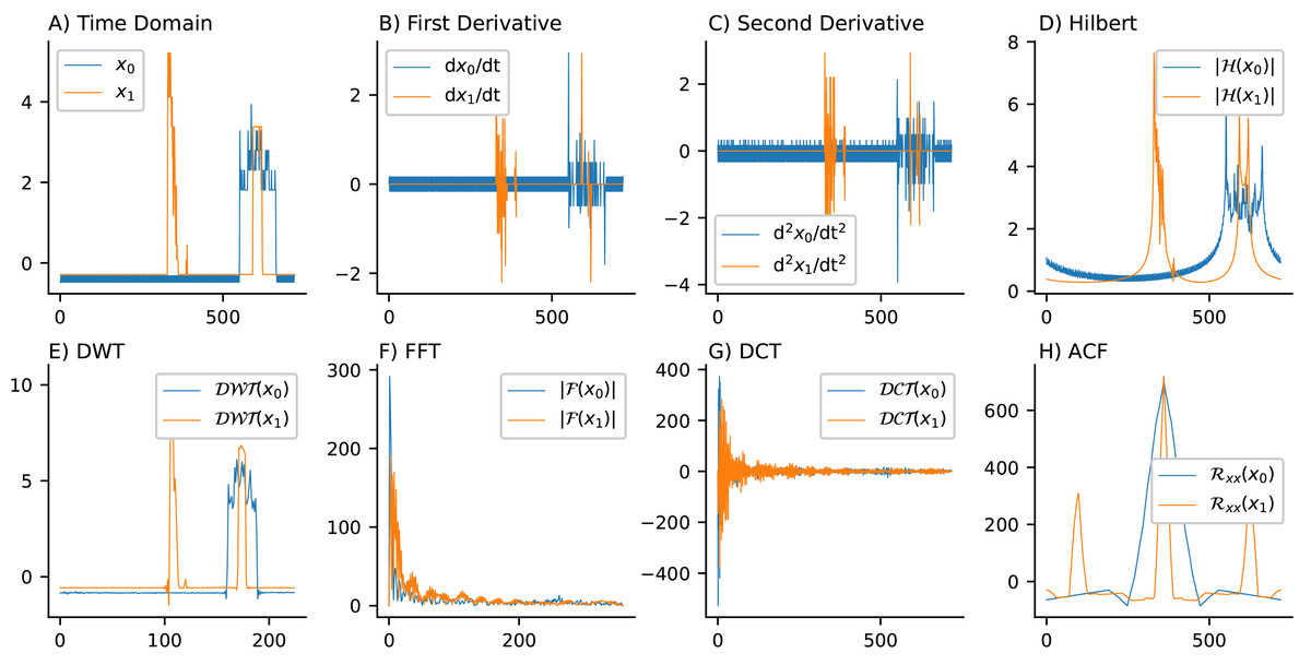
Figure 1: Time series representations for the computers dataset (desktop and laptop classes based on power consumption): The top row displays the (A) time domain, (B) first-order derivative, (C) second-order derivative, and (D) Hilbert transform. The bottom row presents the (E) DWT, (F) FFT, (G) DCT, and (H) ACF representations.
Time domain
The time domain representation captures the raw signal values over time, providing essential information about the sequence of observations in their original form. It is particularly useful for analyzing trends, patterns, and peaks directly from the data.
Given a time series with , the time domain representation comprises the values without any transformation.
First derivative
The first derivative represents the rate of change or slope of the time series, highlighting rapid transitions or trends over time. It helps to identify how the values change from one point to the next.
Mathematically, the first derivative at time can be approximated as:
(1)
If , this simplifies to capturing changes between consecutive time points.
Second derivative
The second derivative captures changes in the rate of change, making it useful for identifying inflection points, peaks, and valleys. In other words, it quantifies how the first derivative (rate of change) itself changes over time, which is related to curvature.
Mathematically, the second derivative can be expressed as:
(2)
This representation is particularly useful for detecting curvature and identifying transitions in the trend.
Hilbert transform
The Hilbert transform provides the analytic signal of a time series, allowing the extraction of instantaneous amplitude, phase, and frequency. This is particularly useful for capturing envelope and phase information, which can distinguish different classes of time series.
The Hilbert transform is defined as:
(3) where P.V. denotes the Cauchy principal value. The resulting analytic signal provides the instantaneous amplitude , and phase . In this study, only the amplitude part is considered.
DWT
DWT decomposes a time series into multiple frequency components at various resolutions, capturing both time and frequency information. This multiresolution analysis is beneficial for identifying localized patterns and features, making it suitable for non-stationary time series.
Mathematically, wavelets express as:
(4) where are the wavelet basis functions at scale and translation , and are the coefficients representing the signal at different resolutions.
Meyer wavelet (Meyer, 1986) was selected in this study as the basis function for decomposing the signal. The Meyer wavelet is unique among wavelets due to its smoothness and the fact that it is defined in the frequency domain, which makes it well-suited for capturing both high and low-frequency components in a signal. In this study, only approximation coefficients at level-2 are used.
FFT
FFT converts the time series into the frequency domain, representing the signal as a sum of sinusoids. It enables the identification of dominant frequencies and periodic structures within the data.
The discrete Fourier transform (DFT) of a time series of length N is given by:
(5)
The FFT is used to efficiently compute this transformation, revealing the frequency components of the time series. The resulting signal consists of the instantaneous amplitude and phase components. Only the amplitude part is considered in this study. Since the time series data is real-valued, is Hermitian-symmetric, and the amplitude is symmetric as well. Therefore, only the first half of the amplitude is of interest, as phase-independent features are captured.
DCT
DCT represents the time series as a sum of cosine functions oscillating at different frequencies, emphasizing energy compaction in a few coefficients. It is often used for compression and highlighting significant patterns.
The DCT of a time series of length N is given by:
(6) This representation effectively captures the essential features of the signal with fewer coefficients.
ACF
Autocorrelation measures the similarity between a time series and lagged versions of itself over different time lags, helping to identify repeating patterns and temporal dependencies.
The autocorrelation function at lag is given by:
(7)
While ACF can reveal periodic structures, it does not explicitly decompose the signal into frequency components like FFT. Instead, periodicity is inferred from peaks in the ACF. According to the Wiener-Khinchin theorem, the power spectral density of a stationary signal is the Fourier transform of its autocorrelation function, establishing a fundamental link between ACF and frequency analysis.
Features in categories
Features in this study are grouped into four categories: norms, stats, series, and temp. Statistical features and norms capture vectorial and distributional aspects, while the series category focuses on the sequence of values. Temporal features highlight interactions over time. This distinction aligns with different time series types—temporal aspects dominate in motion, ECG, EPG, and sensor data, whereas value sequences are more relevant in image data. Most features were selected from Catch22 and TSFresh, except for MLD and P4B, which were newly introduced.
Norms
Norms quantify the magnitude of a vector, offering insights into its scale and behavior across different spaces. They are widely used for comparison, regularization, and measuring similarity or deviation.
The norm sums absolute values, reflecting a grid-like path, while the norm represents the Euclidean distance. The norm captures the largest component, and the norm identifies the smallest. In this study, we incorporate and norms. Instead of using and , we directly consider maximum and minimum values.
Stats
Statistical features describe key aspects of a time series, such as its shape, variability, central tendency, and distribution. These features aid in classification, forecasting, and anomaly detection by summarizing trends and patterns.
The selected features include median, standard deviation, skewness, and kurtosis, while the mean was excluded due to its negligible impact on performance. Additionally, differential entropy, the mode from a 10-bin histogram from Catch22 (HMod), and P4B—a new feature that partitions the series into four equal segments and computes probabilities for each—are incorporated.
Series
This category extracts distinguishing characteristics from value sequences. The selected features are:
MLD calculates the mean of the logarithm of first-order differences. It is newly introduced in this study.
HCP measures large fluctuations by computing the proportion of high incremental changes. Originally used in heart rate variability to count instances where changes in successive normal sinus intervals exceed a threshold (Ewing, Neilson & Travis, 1984). The generalized version calculates the proportion of successive differences exceeding .
LMT records changes in the autocorrelation timescale after incremental differencing.
FMA determines the first minimum of the autocorrelation function.
MTQ calculates the Shannon entropy for consecutive letter pairings in an equiprobable three-letter symbolic sequence.
BML1 measures the longest sequence of consecutive values above the mean.
BML0 finds the longest sequence of successive declines in the series.
WRC calculates the total power in the lowest fifth of frequencies of the Fourier power spectrum.
MIS identifies the initial minimum of the automutual information function.
PWT calculates a periodicity metric with reference to Wang, Wirth & Wang (2007).
DTD fits an exponential curve to a 2-dimensional embedding space at increasing distances.
CAM indicates the number of values in the series that exceed the mean.
MSC determines the mean of the second derivative using a central difference approximation.
FLMn and FLMx indicate the first and last locations of the series’ minimum and maximum values relative to its length.
A total of 10 features were selected from Catch22 and 6 from TSFresh, in addition to MLD.
Temporal
Temporal relations are central in this category. Only time-domain and derivative representations (DT1 and DT2) were considered, as shown in Table 1.
- •
CID is the complexity-invariant distance that estimates complexity for a time series. It relies on the intuition that a more complex time series has more peaks and valleys.
- •
C3 uses the third-order autocovariance, known as c3 statistics, to measure non-linearity in the time series (Schreiber & Schmitz, 1997), given by: (8)
- •
TRAS returns the time reversal asymmetry statistic (Fulcher & Jones, 2014), defined as: (9)
- •
NCM calculates the number of crossings of the time series on value . A crossing occurs when two sequential values shift from below to above or vice versa. Setting to zero returns the number of zero crossings. Here, is set to the mean.
- •
PRD returns the percentage of non-unique data points. Non-unique values appear more than once in the time series. The count of such values is normalized by the total number of points in the series.
Demonstration of incremental feature complementarity
To provide evidence that cross-representation features contribute incrementally useful and non-redundant information, a synthetic-signal experiment was conducted. The signal was designed to contain multiple interpretable components so that the effect of each feature representation could be clearly illustrated. Specifically, each synthetic signal of length was generated as
(10) where controls a linear trend, and define a sinusoidal oscillation, introduces a sharp spike at position , and is Gaussian noise with zero mean and variance . Random variation of the parameters across realizations produced a dataset of 200 heterogeneous, perturbed signals.
For each representation, simple statistical descriptors (e.g., Max, L1, L2) were extracted and compared in an incremental manner. The baseline was defined as the time and frequency (FFT) domain representations, and additional representations were incorporated in the order DT1, DT2, DWT, ACF, DCT, and HLB.
To assess complementarity, two measures were tracked as representations were added incrementally to the feature set. The first measure, Average Incremental Mutual Information (AIMI), quantifies the additional mutual information provided by a new feature with respect to the features already included. The second measure, Variance Ratio (VR), is defined as the cumulative variance explained by a principal component analysis (PCA) model fitted to the integrated feature space, normalized by the variance explained by the baseline (TIME+FFT) features alone.
The results are shown in Fig. 2. With few exceptions, both AIMI and VR consistently increase as additional representations are incorporated in the order {DT1, DT2, DWT, ACF, DCT, HLB}. This demonstrates that each domain contributes incrementally useful and non-redundant information, thereby complementing the baseline. In particular, derivatives emphasize local changes, DWT captures multi-scale dynamics, ACF captures long-range dependencies, DCT capture global oscillatory structure, and the Hilbert transform characterizes instantaneous amplitude and phase. These findings provide empirical justification for the CFIRE framework’s systematic integration of diverse feature representations.
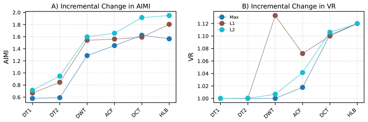
Figure 2: Incremental feature complementarity across representations.
(A) AIMI between a newly added representation and the existing set. (B) Cumulative VR relative to the baseline time-domain feature. Representations are incrementally added in the order: DT1, DT2, FFT, DCT, DWT, ACF, HLB. The results confirm that each added representation contributes complementary information while preserving discriminative power.
Proposition (informal). Let Y be the class label and let be scalar features extracted from pairwise distinct representations of the same signal (e.g., TIME, DT1, DT2, FFT, DCT, DWT, ACF, HLB). Then the total discriminative information carried by the integrated feature vector is nondecreasing with :
and each term with equality if and only if is conditionally independent of Y given (i.e., is redundant with respect to Y given the existing features). In particular, when a new representation reveals a component of the signal that is not a measurable function of the previously used representations (e.g., localized transients captured by DWT that TIME/FFT cannot reproduce), it follows that .
Proof sketch. The chain rule of mutual information yields
Nonnegativity of conditional MI implies monotonicity in . Moreover, if and only if , establishing the redundancy criterion.
To argue strict positivity for cross-representation additions, consider the signal decomposition , where components encode trends, periodicities, localized transients, and long-range dependencies, and denotes noise. Features are formed by measurable functionals on representation operators (e.g., derivative, Fourier, wavelet, Hilbert, autocorrelation). If for some component it holds that retains nonzero Fisher information about Y via while cannot reconstruct (i.e., ), then and by the data-processing inequality and standard identifiability arguments. Examples include (i) DWT capturing localized transients not preserved by global FFT magnitudes, (ii) ACF summarizing long-range dependence not reproduced by pointwise TIME or local derivatives, and (iii) HLB amplitude revealing envelope variations orthogonal to phase-agnostic summaries. Hence, adding features from such representations strictly increases unless they are perfectly redundant.
Finally, the empirical variance ratio (VR) used in Fig. 2 is nondecreasing under feature concatenation because the total PCA variance equals the trace of the sample covariance, which is monotone when appending a nonzero-variance feature and remains unchanged only if the new feature is an exact linear combination of existing ones.
Computational complexity analysis
The computational complexity of the approach is influenced by the costs associated with different representations and features, as various combinations of these elements are utilized. Each component has a distinct computational cost, impacting scalability and processing time, particularly when handling large datasets.
Complexity of representations
No additional cost is incurred for the time domain representation. However, the first and second derivatives require computation based on differences between neighboring time points. Since a linear scan across the series data is performed, the time complexity of this operation is .
The transformation of a time series from the time domain to the frequency domain is carried out using FFT. While the direct computation of the discrete Fourier transform has a complexity of , FFT reduces this complexity to , making it more efficient.
The HLB requires convolution with a kernel function. When performed using FFT-based convolution, the complexity remains , making it efficient for long time series.
The DWT is applied to compute multiscale decompositions of the time series. For most implementations (such as Meyer, Haar, or Daubechies wavelets), the complexity is , as filters are recursively applied over progressively coarser scales.
Similar to FFT, the DCT transforms a time series into the frequency domain with a focus on energy compaction. Since its computational complexity is also , it is effective for tasks involving compression and decorrelation.
The ACF requires computing correlations between a time series and its lagged versions. A naive computation results in complexity, but by utilizing FFT-based approaches, this can be reduced to .
Complexity of feature calculation
The complexity of computing norm and statistical features (such as , , min, max, median, variance, and skewness) is linear with respect to the time series length . For example, the median can be computed with a single pass through the data, resulting in a complexity of .
The Catch22 feature set has been designed for computational efficiency, with most features exhibiting complexity. However, some features in TSFresh, such as sample_entropy, lempel_ziv_complexity, and fft_aggregated, have higher computational costs. Depending on their implementation, certain TSFresh features may have a complexity of or higher. To mitigate computational costs, features with greater complexity were explicitly excluded from TSFresh. The majority of selected features, including CAM, NCM, MSC, and the first and last locations of extrema, have a complexity of .
The recently introduced P4B feature, which segments the time series into four equal-length bins and determines the probability for each, also has a linear complexity of . This is achieved by scanning the time series and counting occurrences within each bin.
The newly introduced MLD feature, which computes the mean of the logarithm of first-order differences, consists of three operations: computing first-order differences, taking their logarithms, and computing the mean. Since each step requires operations, the overall complexity remains .
A summary of complexity is provided in Table 2. Multiple features are computed for each time series representation in this study. Since both feature calculations and transformations have an approximate complexity of , the total complexity for computing all features for a single representation remains . The overall computational complexity is given by , where denotes the length of the time series, represents the number of distinct representations, and refers to the number of features per representation. Additionally, feature calculations for each representation can be executed in a highly parallelized manner, reducing the effective computational cost. Despite the theoretical complexity increasing linearly, practical execution time is significantly optimized due to this parallelism.
| Representations | Complexity | Features | Complexity |
|---|---|---|---|
| DT1 and DT2 | Norms | ||
| HLB | Stats | ||
| DWT | P4B | ||
| FFT | Catch22 | Mostly | |
| DCT | TSFresh | Mostly | |
| ACF | MLD |
Classifier
Following the approach in Cabello et al. (2024) and Dempster, Schmidt & Webb (2024), extremely randomized trees (ET) (Geurts, Ernst & Wehenkel, 2006) were employed as the classifier after extracting features using CFIRE. In ‘Classifiers Evaluation’, the classification performance of ET is shown to be superior to that of RF (Breiman, 2001), RoF (Rodriguez, Kuncheva & Alonso, 2006), ridge regression classifier, CART (Breiman et al., 1984), support vector machines (SVM) (Hearst et al., 1998), and eXtreme Gradient Boosting (XGB) (Chen & Guestrin, 2016).
ET is an ensemble ML technique that constructs multiple decision trees during training, similar to RF. This method is applicable to both classification and regression tasks. A vast number of unpruned decision trees are generated using a randomly selected threshold for each split and a randomly chosen subset of features for evaluation. In regression tasks, the final prediction is obtained by averaging the outputs of all trees, while in classification, a majority vote determines the outcome.
Despite similarities with RF, ET differs in two key aspects. First, tree splits in RF are deterministic, whereas in ET, they are entirely random. Second, bootstrapping is applied in RF, where observations are drawn with replacement, leading to repeated samples. In contrast, ET draws observations without replacement, preventing repetition. This additional randomness accelerates training by eliminating the need to compute the most optimal feature split.
Three primary hyperparameters require tuning during the training process: the number of decision trees in the ensemble, the number of input features randomly selected and evaluated at each split, and the minimum number of samples required in a node to generate a new split. By default, a minimum of two samples is needed in a node for a split to occur. According to Dempster, Schmidt & Webb (2024), the number of trees (or estimators) is fixed at 200. This choice is further supported by the sensitivity analysis presented in ‘Classifiers Evaluation’, where varying tree counts were evaluated.
The square root of the total number of features is typically recommended as the number of input features to be randomly selected (Geurts, Ernst & Wehenkel, 2006). However, Dempster, Schmidt & Webb (2024) demonstrated that selecting 10% of the total features is more effective. In this study, this proportion was further increased to 15% to identify the best split, as CFIRE yields approximately 200 features. This adjustment proved beneficial, even though the increase in Dempster, Schmidt & Webb (2024) was due to their larger feature set.
Performance evaluation
Performance evaluation during representation and feature selection was conducted using 5-fold cross-validation, with accuracy (ACC) as the evaluation metric. For comparisons with SOTA methods, Monte Carlo cross-validation was employed, utilizing 30 predefined resamples based on the indices provided by Middlehurst, Schäfer & Bagnall (2024). The difference in mean accuracy and the pairwise win/draw/loss results between CFIRE and other methods were reported using a multiple comparison matrix (MCM) (Ismail-Fawaz et al., 2023). Additionally, a critical difference diagram (CDD) (Ismail Fawaz et al., 2019) was used to compare the average ranks of different methods. Pearson correlation analysis was applied to examine the relationship between various factors and the performance improvements achieved by CFIRE over other approaches.
When comparing feature-based methods, additional metrics were included to capture complementary aspects of classification performance:
Balanced accuracy (BALACC): The arithmetic mean of class-wise accuracies, mitigating bias in imbalanced datasets.
F1-score: The harmonic mean of precision and recall, providing a balanced measure of sensitivity and positive predictive value.
Area under the receiver operating characteristic (ROC) curve (AUC): Evaluates the ability of the classifier to discriminate between classes across thresholds.
Negative log-likelihood (NLL): Measures the quality of probabilistic predictions, with lower values indicating better calibrated models.
Compute time was assessed using an Intel i7-11700 @2.50 GHz CPU with 8 cores and 32 GB RAM.
Experiments
The experimental evaluation was designed to comprehensively assess the effectiveness and scalability of CFIRE. In line with the central hypothesis that combining diverse representations with optimized feature selection improves, six sets of experiments were conducted. First, a sensitivity analysis was carried out to study the interaction between representations and features and to identify optimal configurations. Second, the performance of the designated classifier within CFIRE was compared against alternative classifiers, including parameter sensitivity. Third, CFIRE was evaluated against established feature-based approaches. Fourth, benchmarking against SOTA methods in was undertaken. Fifth, the scalability of CFIRE to ultra-long sequences was investigated through synthetic length sweep experiments. Finally, robustness to varying sequence lengths was tested via length invariance experiments, in which the baseline model was trained on the intact ultra-long sequence of points, while in fragmented regimes either training or testing sequences were split into shorter fragments (ranging from to points) with the other side kept unfragmented.
Sensitivity analysis
Representation and feature optimization
Following the construction phase, ablation and isolation analyses were conducted within the CFIRE pipeline to identify optimal combinations of representations and features. The impact of various configurations was visualized using 3D bar graphs to illustrate the ACC obtained across different configurations, including (1) ablation of both representations and features, (2) ablation of representations with isolation of features, (3) isolation of representations with ablation of features, and (4) isolation of both representations and features. The “None” tick label on the representation (x-axis) and feature (y-axis) axes indicates that no ablation or isolation was applied.
Norms category (Fig. 3A): With a baseline ACC of 0.8166, the analysis revealed that removing DT1 or DCT from representations and L1 or Min from features significantly decreased performance, highlighting their importance. Conversely, eliminating FFT and L2 resulted in the highest ACC (0.8204), suggesting their minimal contribution. Isolation experiments confirmed the benefit of synergy, as individual elements generally performed worse than when combined. DWT, DCT, L1, and Max showed strong standalone capabilities, while FFT, DT2, and L2 relied on complementary elements.
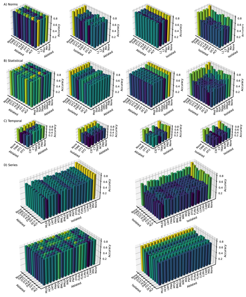
Figure 3: Sensitivity analysis of representations and features across the following categories: (A) norms, (B) statistical, (C) temporal, and (D) series.
The plots show the ACC for four configurations: (1) ablating both representations and features, (2) isolating representations while ablating features, (3) ablating representations while isolating features, and (4) isolating both representations and features.
Statistics category (Fig. 3B): Starting with a mean ACC of 0.8443, removing DifEn, P4B, DT1, DWT, or DCT caused significant performance drops, emphasizing their importance. The highest ACC (0.8491) was achieved when both HMod and FFT were eliminated. Isolation again highlighted the importance of synergy, though P4B, DWT, ACF, and TIME showed relatively good individual performance.
Series category (Fig. 3D): With a baseline ACC of 0.8588, removing LLMx, PWD, BML1, LLMn, DT2, or FFT had a positive effect, while removing DTD, MSC, DWT, or TIME led to a decline. Synergy was again crucial, and the full set yielded the best results. Notably, removing FLMn and DT2 resulted in the highest ACC (0.8620), suggesting potential noise or redundancy. CAM, WRC, MLD, TIME, HLB, and DWT performed well in isolation, whereas FLMn, DT2, and BMQ did not.
Temporal category (Fig. 3C): Starting with a mean ACC of 0.8431, ablation generally decreased performance, with TIME and C3 removals having the largest negative impact. The highest performance was consistently achieved with the full set of features and representations.
Across all categories, the analysis demonstrated that using multiple representations enhanced performance compared to relying solely on TIME. In certain cases, removing specific representations slightly improved ACC, particularly evident in the isolation analysis. This highlights the advantage of diverse representations, enabling feature extraction multiple times.
While the full feature set from the construction phase generally improved performance, eliminating redundant or less informative pairs—identified through sensitivity analysis—further enhanced ACC. The series category had the most significant impact on classification performance (0.8620), followed by statistics (0.8491), temporal (0.8431), and norms (0.8204), with a combined ACC of 0.8708.
Following the elimination phase, the norms, statistics, series, and temporal categories retained three, six, 16, and five features, respectively, and seven, seven, seven, and three representations, respectively, resulting in a total of 190 features (21 norms, 42 statistics, 112 series, and 15 temporal).
Overall, the analysis confirmed that while individual features and representations contribute to predictive performance, the full set of extracted features and representations yields the best results.
Dataset-specific representation sensitivity
To complement the general representation and feature optimization analysis, a dataset-specific perspective is provided in Fig. 4. The figure contrasts isolation (solo) and ablation results across two representative datasets: FordB, characterized by periodic oscillations, and GunPoint, which is dominated by aperiodic gesture-like patterns.
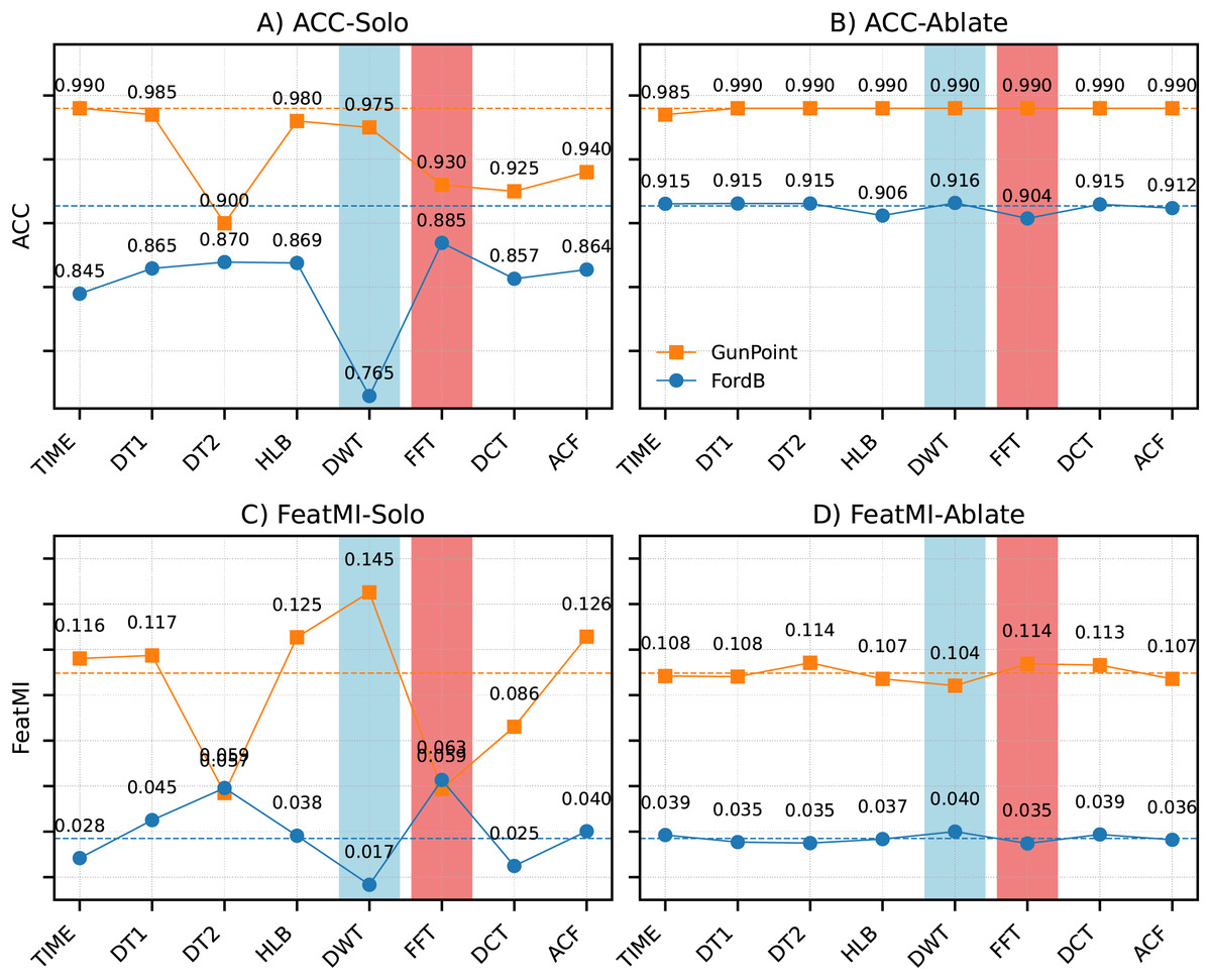
Figure 4: Comparison of isolation (A, C) and ablation (B, D) results for FordB (periodic) and GunPoint (aperiodic).
The differences in (A and B) ACC and (C and D) feature–label mutual information (FeatMI) are presented. Rows correspond to ACC and feature–label mutual information (FeatMI). Dashed lines indicate the baseline using all representations (ALL). Fourier features dominate for FordB, consistent with its global periodic oscillations, whereas wavelet features dominate for GunPoint, reflecting the localized transient nature of gesture-like signals.
For FordB, the FFT representation produced the highest solo ACC ( ), substantially outperforming the discrete wavelet transform (DWT) ( ). This behavior is consistent with the global periodic structure of FordB, which is well aligned with the frequency decomposition captured by Fourier features. Conversely, GunPoint demonstrated the opposite trend: DWT dominated in the solo setting ( ), while FFT lagged behind ( ). The superiority of wavelet-based features can be attributed to the localized and transient nature of gesture signatures, which are more effectively captured by time–frequency methods than by global Fourier analysis.
Ablation experiments revealed that the removal of individual representations had minimal effect. For FordB, ACC with all representations (ALL: ) was nearly identical to the ablation cases ( ). Similarly, GunPoint performance remained unchanged (ALL: vs. ablations: ). These results suggest that discriminative information is distributed across multiple representations and reinforced through redundancy. The complementary contributions are further supported by feature–label mutual information (FeatMI), which indicates that useful signal is not confined to a single transformation but is instead distributed across multiple transformations.
Classifiers evaluation
To determine the most effective classifier for the extracted features, the performance of ET was first evaluated with varying tree counts ranging from 50 to 1,000. Subsequently, ET was compared against widely used classifiers, including RF, RoF, XGB, Ridge, CART, and SVM with RBF kernel. Runtime efficiency was evaluated based on the total compute time measured across datasets in the development set.
The relationship between the number of trees in the ET classifier and its performance metrics (ACC, AUC, F1-score) and computational time is shown in Fig. 5. Performance gains were observed with increasing tree counts below 300 but plateaued beyond that point, suggesting that additional trees contribute marginal gains. The increase in performance was accompanied by a linear rise in computational time, demonstrating that while a higher number of trees enhances predictive power, it also increases computational overhead.
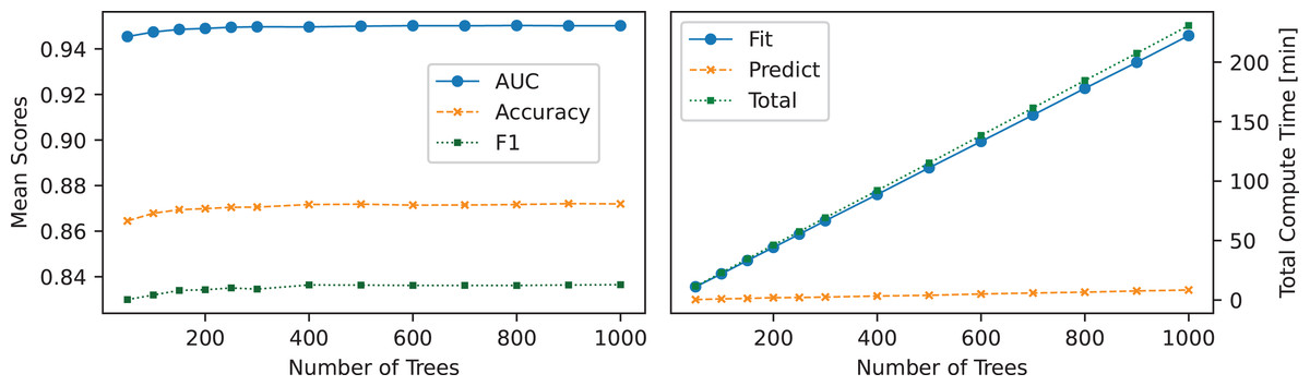
Figure 5: Effect of tree count on ET: the left panel shows the number of trees used vs. mean scores, while the right panel illustrates the number of trees used vs. total compute time.
In addition to evaluating tree count effects, a comparative analysis of classifiers was conducted to assess trade-offs between computational efficiency and classification performance. Figure 6 illustrates these trade-offs by comparing mean scores and compute times across the classifiers. Among the classifiers evaluated, ET achieved the highest mean classification scores, emerging as the most effective feature-based TSC classifier. RF and RoF exhibited performance levels comparable to ET but with slightly lower computational efficiency. XGB provided a balanced trade-off, demonstrating moderate computation times while maintaining strong classification performance. In contrast, Ridge, CART, and SVM achieved lower classification accuracy but offered significantly faster computation times. The results highlight ET as the most effective model for feature-based TSC, balancing classification performance and computational efficiency. However, alternative classifiers such as XGB present viable trade-offs, particularly in resource-constrained environments.
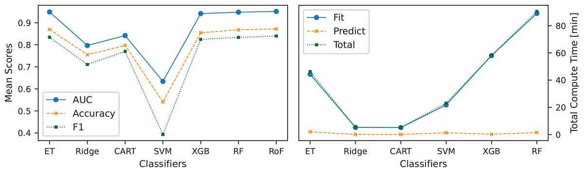
Figure 6: Analysis of CFIRE classifiers: evaluating the balance between classification accuracy and computational cost by comparing mean scores and compute times across different classifiers used with CFIRE.
Comparison with feature based methods
In feature-based classification, including CFIRE, an ML classifier operates on features derived from time series data. For these experiments, the ET classifier was used with consistent configurations and a fixed random seed of zero for reproducibility. Results for other feature-based methods were replicated using the aeon toolbox (Middlehurst et al., 2024). Although Quant is not a feature-based approach, it was included in the compute time analysis as a benchmark for efficiency and effectiveness.
CDD illustrating the relative effectiveness of different feature-based methods in TSC is presented in Fig. 7. The results indicate CFIRE as the top performer with the lowest average rank (2.0880), significantly outperforming FreshPRINCE (2.2465) and other methods. The MCM in Fig. 8 confirms CFIRE’s superiority over FreshPRINCE and others with predominantly negative mean-difference values and significant p-values.
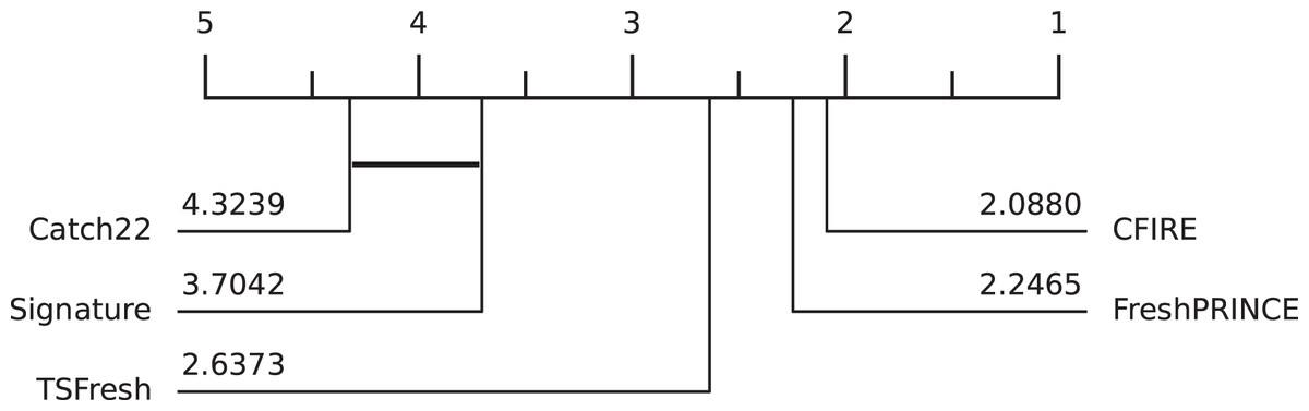
Figure 7: Comparison of feature-based methods and CFIRE: CDD illustrating the performance ranking of CFIRE against other feature-based classification methods.
Lower ranks indicate better overall performance.
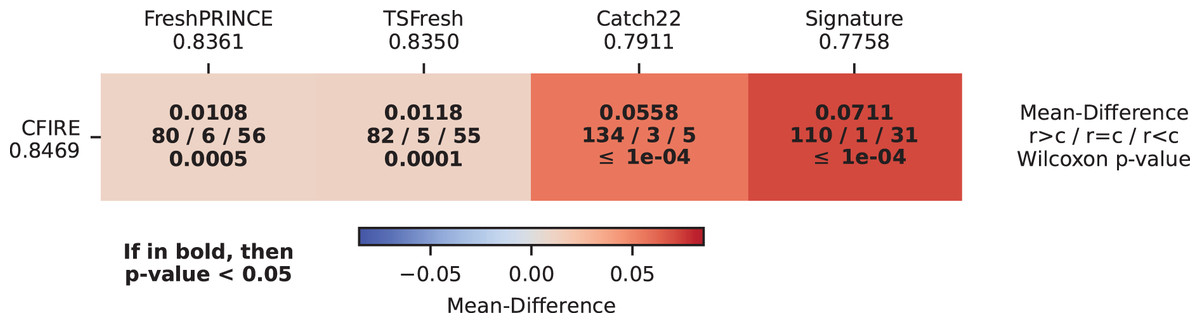
Figure 8: Pairwise performance comparison of feature-based methods and CFIRE: MCM showing the mean ACC differences between CFIRE and other feature-based classifiers, with statistical significance highlighted.
A summary of the average performance metrics for feature-based classifiers is presented in Table 3. The results show that CFIRE consistently achieved the highest scores across all key metrics. In terms of ACC, CFIRE attained the highest value (0.844), surpassing FreshPRINCE (0.836) and TSFresh (0.835). The BALACC for CFIRE was 0.817, indicating its robustness in handling class-imbalanced datasets. Furthermore, CFIRE recorded the highest AUC at 0.950, demonstrating its strong discrimination ability. With the lowest NLL of 0.567, CFIRE provided superior probabilistic predictions compared to other classifiers. Lastly, in terms of F1-score, CFIRE again outperformed all competitors, achieving 0.815, which reflects its effective balance between precision and recall.
| Classifiers | ACC | BALACC | AUC | NLL | F1 |
|---|---|---|---|---|---|
| CFIRE | 0.847 (1) | 0.822 (1) | 0.951 (1) | 0.537 (1) | 0.815 (1) |
| FreshPRINCE | 0.836 (2) | 0.801 (3) | 0.948 (2) | 0.606 (2) | 0.806 (2) |
| TSFresh | 0.835 (3) | 0.807 (2) | 0.948 (2) | 0.608 (3) | 0.805 (3) |
| Catch22 | 0.791 (4) | 0.764 (4) | 0.927 (4) | 0.704 (4) | 0.761 (4) |
| Signature | 0.776 (5) | 0.748 (5) | 0.912 (5) | 0.869 (5) | 0.746 (5) |
A pairwise mean ACC comparison between CFIRE and FreshPRINCE is depicted in Fig. 9, which provides insights into their relative performance across datasets with varying class distributions and time series lengths. The analysis indicates that CFIRE outperformed FreshPRINCE in 80 datasets, while FreshPRINCE achieved better results in 56 datasets. Notably, CFIRE’s performance advantage became more pronounced as dataset characteristics, such as class count and sequence length, increased. This suggests that CFIRE provides stronger generalization capabilities in complex classification tasks.
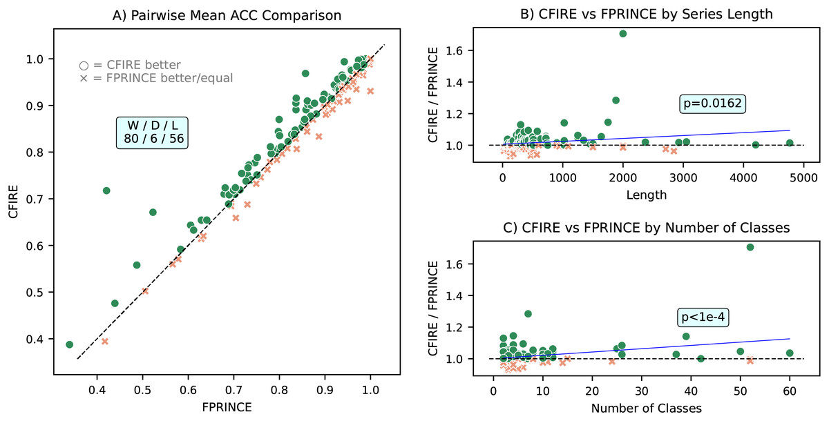
Figure 9: Comparative performance analysis of CFIRE and FreshPRINCE.
(A) Pairwise mean ACC comparison showing CFIRE’s performance relative to FreshPRINCE across all datasets. (B) Ratio of CFIRE to FreshPRINCE ACC as a function of time series length, indicating CFIRE’s increasing advantage with longer sequences . (C) Ratio of CFIRE to FreshPRINCE ACC as a function of the number of classes, showing enhanced performance for CFIRE in datasets with more classes .
An analysis of computational efficiency is provided in Fig. 10, where the runtime of CFIRE is compared with other feature-based classifiers, including Quant—the fastest method among SOTA approaches. The comparison considers the total time required for feature transformation, model training, and prediction. To enhance performance, CFIRE’s feature extraction stage was implemented with parallel processing, significantly reducing computation time. Similarly, other baseline methods were executed using parallelization options provided by scikit-learn to ensure a fair comparison. CFIRE demonstrated computational efficiency comparable to Quant, indicating that it delivers superior performance without incurring excessive computational costs. This efficiency is particularly valuable when scaling to large datasets, where computational overhead can become a limiting factor.
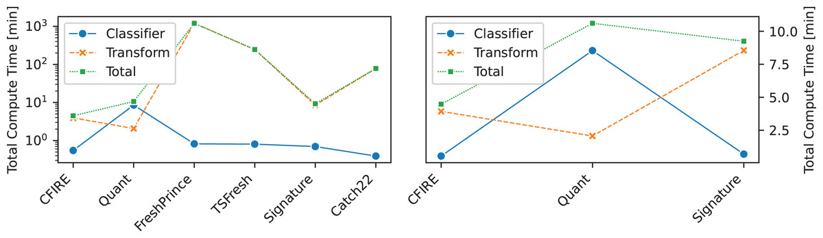
Figure 10: Compute times comparison between CFIRE and feature-based methods.
Quant, the fastest method among the SOTA in all categories, is also included in the comparison.
Among other feature-based methods, CFIRE consistently outperformed FreshPRINCE, TSFresh, and Catch22 in terms of speed. While FreshPRINCE and TSFresh exhibited reasonable performance, their feature extraction processes were more computationally intensive. Catch22, despite its relatively simple feature extraction mechanism, failed to match CFIRE’s efficiency. These results underscore the optimized nature of CFIRE’s feature extraction pipeline.
Comparison with state of the art
CFIRE was also compared with leading TSC methods, each representing a distinct category of approaches. The selected methods include HC2, MR-Hydra, RDST, WEASEL-2, H-InceptionTime, Quant, FreshPRINCE, and PF, which correspond to hybrid, convolutional, shapelet-based, dictionary-based, deep learning, interval-based, feature-based, and distance-based classifiers, respectively. The results for these methods were obtained from Middlehurst, Schäfer & Bagnall (2024), with the exception of Quant, for which results were reproduced using the aeon toolkit.
As illustrated in Fig. 11, CFIRE’s ranking among SOTA methods reveals its comparable performance to Quant, with no statistically significant difference observed. This positions CFIRE within the top-tier classifiers, following the computationally intensive HC2 and MR-Hydra.
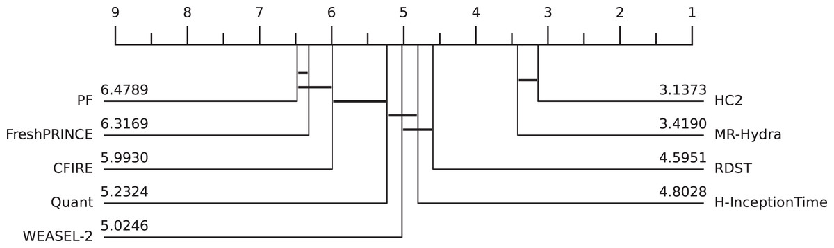
Figure 11: Comparison of SOTA TSC Methods and CFIRE: CDD illustrating the performance rankings of CFIRE against leading TSC methods across different classification paradigms.
Lower ranks indicate better overall performance.
Further analysis using an MCM is presented in Fig. 12, which provides a pairwise performance comparison between CFIRE and other SOTA classifiers. While HC2, MR-Hydra, RDST, WEASEL-2, and H-InceptionTime outperformed CFIRE, the Wilcoxon p-values for these comparisons were below 0.05, indicating statistically significant differences. However, in the comparison between CFIRE and Quant, the p-value exceeded 0.05, confirming that their performances were statistically indistinguishable. CFIRE outperformed both FreshPRINCE and PF, which represent the feature-based and distance-based classification paradigms, respectively.
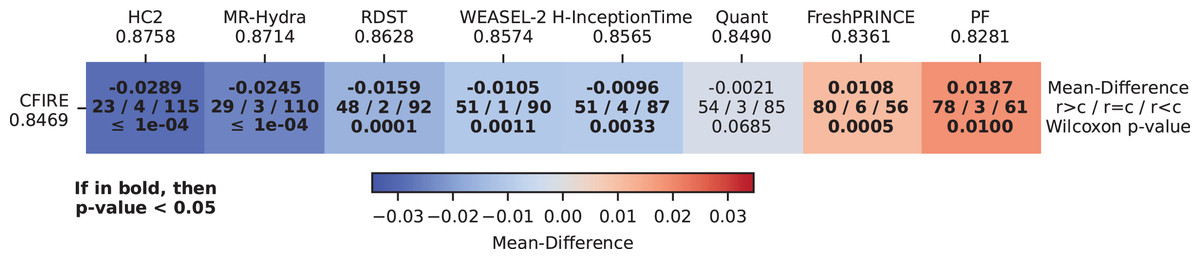
Figure 12: Pairwise performance comparison of SOTA TSC methods and CFIRE: MCM illustrating the mean ACC differences between CFIRE and various SOTA TSC methods across different classification paradigms, with statistical significance highlighted.
A more detailed pairwise ACC comparison between CFIRE and Quant is provided in Fig. 13. The results show that CFIRE outperformed Quant in 53 datasets while underperforming in 85 datasets. Notably, CFIRE’s relative performance improved as the length of the time series and the number of classes increased, with both relationships exhibiting statistical significance . These findings indicate that CFIRE is particularly well-suited for datasets with complex class structures and longer time series sequences, where it maintains a robust classification advantage.
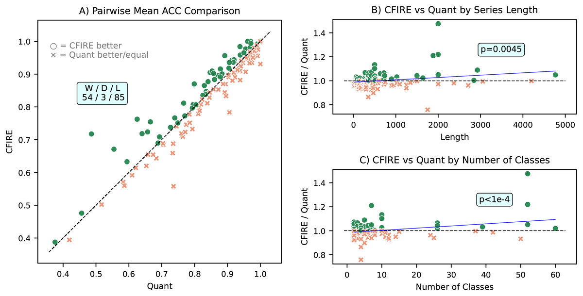
Figure 13: Comparative performance analysis of CFIRE and Quant: (A) Pairwise mean ACC comparison illustrating CFIRE’s performance relative to Quant across all datasets. (B) ACC ratio of CFIRE to Quant as a function of time series length, demonstrating CFIRE’s increasing advantage for longer sequences . (C) ACC ratio of CFIRE to Quant based on the number of classes, highlighting CFIRE’s improved performance in datasets with more classes .
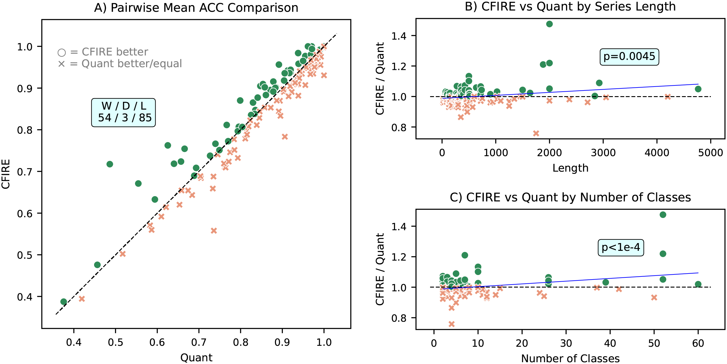
Scaling to ultra-long sequences
To assess the scalability of CFIRE to ultra-long sequences, synthetic time series with increasing lengths from to were evaluated. Performance metrics (ACC, F1, Balanced ACC, AUC, and NLL) and runtimes for each stage of the pipeline were recorded.
As shown in Fig. 14 (left: classification, right: runtime), classification performance improved moderately with longer sequences (e.g., ACC rising from at to at , AUC from to ). At the same time, runtimes for the transformation phase scaled nearly linearly with sequence length (e.g., 5 s at 5 k vs. 460 s at 100 k), in agreement with the theoretical complexity of . Notably, training and prediction times remained nearly constant, demonstrating that the computational bottleneck lies in the representation stage.
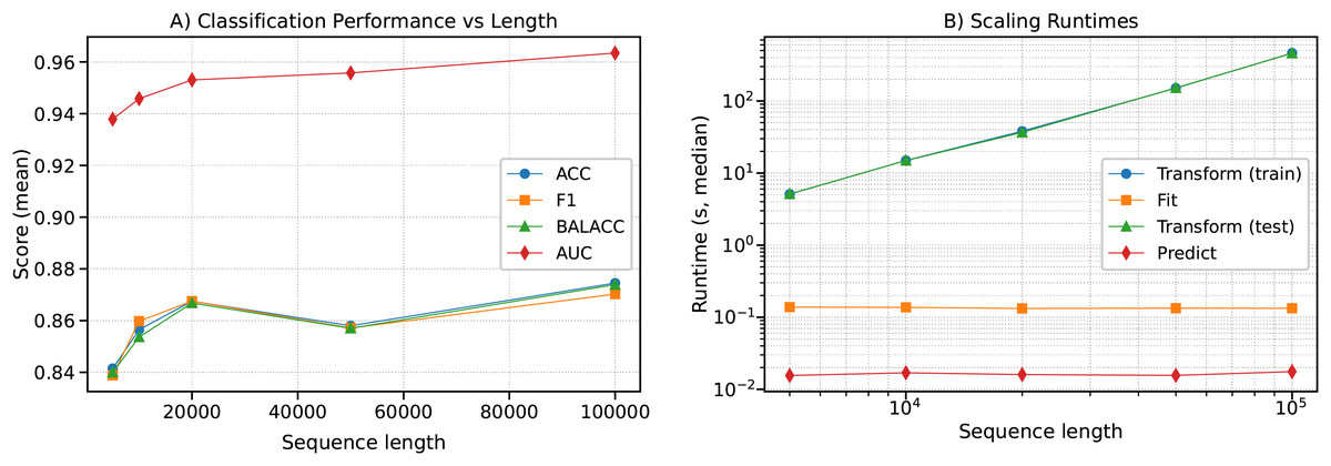
Figure 14: Scaling behavior of CFIRE on synthetic ultra-long sequences.
(A) Classification performance (ACC, F1, Balanced ACC, and AUC) as a function of sequence length. (B) Median runtimes for transformation, fitting, test transformation, and prediction phases. The results empirically validate the theoretical complexity of , showing near-linear growth of transformation costs with sequence length .
Length invariance via fragmentation
In addition to raw scaling, a fragmentation study was conducted to test length invariance. The intact ultra-long sequence ( ) was used as the baseline, while both training and testing sets were fragmented into shorter subsequences of length to . Results are presented in Table 4.
| Fragment length | Train fragmentation ACC | Test fragmentation ACC |
|---|---|---|
| 1,000 | 0.8200 | 0.6775 |
| 5,000 | 0.8550 | 0.7700 |
| 20,000 | 0.8900 | 0.8700 |
| 50,000 | 0.9125 | 0.9150 |
When training on fragments, performance was stable even with moderate reductions in fragment length. For example, training on fragments of length achieved an ACC of , while fragments of nearly matched the baseline ( vs. ). Test fragmentation was more detrimental, with ACC dropping to for fragments of length , but near-baseline performance was restored for fragments of length . These findings suggest that CFIRE preserves classification ability under fragmentation, provided that sufficient temporal context is retained.
Discussions
Complementarity of representations. CFIRE relies on the complementarity of multiple representations, since identical features are systematically extracted under different signal transformations. Derivative-based features emphasize rapid changes in the signal that may be obscured in global spectral summaries. Autocorrelation features capture repeating temporal structures, revealing periodic or quasi-periodic patterns beyond what FFT or DCT coefficients provide. Hilbert transform features encode instantaneous amplitude and phase information, offering a perspective orthogonal to both time- and frequency-domain statistics. By integrating these cross-representation features, CFIRE constructs a multi-perspective representation that preserves discriminative power while minimizing redundancy. The mathematical demonstration in ‘Demonstration of incremental feature complementarity’ further supports this finding, confirming that cross-representation features provide non-redundant, incrementally useful information, thereby offering a theoretical basis for the observed performance gains.
General strengths of CFIRE. The experiments highlight several strengths of the CFIRE framework. Integrating diverse representations yields a more comprehensive feature space, enabling more robust pattern capture across heterogeneous time series. Feature selection and optimization play a central role in reducing redundancy and noise, ensuring that the classifier emphasizes the most informative dimensions. Sensitivity analyses reinforce this observation, demonstrating that representation diversity has a collaborative effect on classification performance. Comparative analysis against other feature-based methods further confirms that CFIRE captures complementary aspects of the data more effectively than single-representation approaches.
Dataset-specific insights. The comparison between FordB and GunPoint illustrates how representational effectiveness depends on dataset characteristics. FordB, with strongly periodic oscillatory dynamics, benefited most from Fourier features, which emphasize global frequency components. GunPoint, by contrast, contains gesture-like, aperiodic variations and exhibited stronger performance with wavelet and derivative features, which emphasize localized and transient structures. Autocorrelation and Hilbert features contributed complementary perspectives in both cases, capturing dependencies and instantaneous variations not represented by conventional domains. Ablation studies showed that no single representation was indispensable: performance remained stable even when individual domains were removed. This robustness underscores both redundancy and complementarity, while highlighting that the relative contribution of each domain is dataset dependent.
Efficiency, scalability, and interpretability. CFIRE achieves statistically significant accuracy gains compared to FreshPRINCE and other feature-based methods, as confirmed by the MCM in Fig. 8. Beyond accuracy, CFIRE provides a distinctive efficiency advantage: feature extraction across representations is parallelized, allowing higher accuracy without substantial computational overhead. This balance of speed and performance distinguishes CFIRE from prior feature-based approaches, where improved accuracy typically incurred longer computation times.
Although CFIRE ranked seventh among nine SOTA methods, it demonstrated strong computational efficiency, closely matching Quant in runtime. According to Middlehurst, Schäfer & Bagnall (2024), Quant remains the fastest method, outperforming the second-fastest by nearly an order of magnitude and surpassing HC2 (the most accurate method) by several orders. CFIRE achieves a favorable trade-off between accuracy and efficiency, making it practical and scalable for large-scale tasks. Each representation (FFT, wavelet, derivative, etc.,) is computed independently, distributing feature extraction without sequential dependency. This design enables near-linear runtime scaling with sequence length and explains why CFIRE maintains speed comparable to Quant despite handling multiple transformations. Its efficiency stems from the parallel execution of low-complexity, pre-defined transformations, minimizing overhead. Unlike deep learning methods that require multiple forward passes through large networks, CFIRE preserves both predictive performance and scalability.
In addition to runtime efficiency, CFIRE demonstrated robustness as the data complexity increased. Pairwise comparisons revealed that its performance was significantly better than both FreshPRINCE and Quant when the sequence length and the number of classes increased. This finding indicates that CFIRE not only maintains efficiency but also scales favorably in terms of predictive accuracy under more demanding classification settings. The ability to retain accuracy advantages as problem dimensionality grows further strengthens its suitability for large-scale and complex time series applications.
CFIRE also provides strong interpretability. Extracted features are organized into structured categories, including norms, statistics, temporal dynamics, and series-based descriptors, with the latter further divided into spectral, autocorrelation, and derivative-based descriptors. When these features are computed under multiple representations, a multilayered and multifaceted view of the data is obtained, revealing both within-domain patterns (e.g., dominant frequencies or autocorrelation structures) and cross-domain correspondences (e.g., spectral features derived from both wavelet and Fourier representations). This structured, multi-representation design enables domain-level insights that are not accessible in black-box SOTA models, illustrating how CFIRE simultaneously achieves interpretability, accuracy, and computational efficiency.
Scalability with sequence length. Experiments confirmed near-linear scaling with sequence length, consistent with the theoretical complexity of . Training and prediction times remained stable, with computational overhead confined to the representation step. Importantly, classification performance slightly improved with longer inputs, suggesting that richer temporal information enhances discrimination.
Fragmentation and streaming scenarios. The fragmentation experiments revealed that CFIRE is partially invariant to sequence segmentation. Training on shorter fragments produced only modest reductions in accuracy, while test-time fragmentation was more harmful. However, when fragments of at least half the sequence length ( points) were preserved, accuracy was nearly indistinguishable from the baseline. This indicates that CFIRE can remain effective in streaming or segmented-data scenarios, provided sufficiently long subsequences are available.
Limitations and future directions
Although CFIRE exhibits favorable trade-offs between accuracy, scalability, and interpretability, several limitations remain. First, while multiple representations are systematically integrated, the selection of representations has been restricted to a predefined set (time, derivative, Fourier, wavelet, autocorrelation, and Hilbert). It is possible that additional representations—such as recurrence quantification, shapelets, or learned embeddings—could further enhance performance. Future work may investigate adaptive mechanisms that dynamically select or weight representations based on dataset characteristics.
Second, although feature selection strategies were employed to mitigate redundancy, the feature space remains high-dimensional. While this dimensionality was managed in the current study, scalability to extremely large datasets or streaming contexts may still present challenges. Incorporating more advanced selection techniques, such as mutual information-based redundancy reduction or sparsity-inducing regularization, may further improve efficiency without compromising discriminative power.
Third, although CFIRE was compared with a broad range of SOTA methods, the evaluation was confined to publicly available benchmark datasets. Additional validation on domain-specific, real-world datasets—such as industrial sensor readings, medical time series, or financial data—would provide stronger evidence of generalizability and practical utility.
Finally, while interpretability is enhanced relative to deep learning-based methods, the granularity of explanations is still constrained by the nature of hand-crafted features. Future research could explore hybrid designs that combine CFIRE’s structured, interpretable feature space with complementary deep representations, thereby unifying interpretability and representation learning in a single framework.
Conclusions
This study introduced CFIRE, a feature-based framework for that integrates multiple representations and organizes features into a structured, interpretable taxonomy. By combining diverse transformations with principled feature selection, CFIRE delivers competitive accuracy while offering clear advantages in efficiency, scalability, and interpretability.
Although CFIRE does not always surpass methods in raw accuracy, it consistently outperforms feature-based baselines and demonstrates robustness to longer sequences, larger class counts, and varied segmentations. These qualities make it a practical solution for real-world applications where accuracy, speed, and interpretability must be balanced. Future extensions to regression, forecasting, and anomaly detection could further expand its impact across scientific and industrial domains.