MPV: a density-peak-based method for automated cluster number detection
- Published
- Accepted
- Received
- Academic Editor
- Luigi Di Biasi
- Subject Areas
- Algorithms and Analysis of Algorithms, Artificial Intelligence, Data Science, Optimization Theory and Computation, Theory and Formal Methods
- Keywords
- Cluster number determination, Peak density, Minimum distance, Automated k detection, Change-point analysis
- Copyright
- © 2025 He and Zhang
- Licence
- This is an open access article distributed under the terms of the Creative Commons Attribution License, which permits unrestricted use, distribution, reproduction and adaptation in any medium and for any purpose provided that it is properly attributed. For attribution, the original author(s), title, publication source (PeerJ Computer Science) and either DOI or URL of the article must be cited.
- Cite this article
- 2025. MPV: a density-peak-based method for automated cluster number detection. PeerJ Computer Science 11:e3315 https://doi.org/10.7717/peerj-cs.3315
Abstract
Unsupervised clustering algorithms have been extensively applied in various research fields. In cluster analysis, determining the best cluster number k is significant. At present, many cluster validity indices (CVIs) have been proposed, including the Calinski-Harabaz index, silhouette index, and Dunn index. However, these CVIs are not effective in determining k for ring, semi-ring, and manifold data sets. We propose MPV (minimum distance and peak variation), a density-peak-based method for automated k detection. It constructs a separation measure through a dual mechanism: (1) distances between density peaks and (2) minimum distances between clusters, while using the maximum intra-cluster minimum distance to model compactness. The optimal for ring, semi-ring, and flow datasets is determined by detecting the largest change in the separation measure sequence. Experiments on 28 synthetic and real-world datasets demonstrate MPV’s accuracy in determining k for complex structures.
Introduction
Cluster analysis is an unsupervised learning algorithm in data mining (Jain, 2010). Clustering classifies samples based on their similarity. Specifically, samples within a cluster should be as similar as possible, while samples between different clusters should be as dissimilar as possible. In recent decades, numerous clustering algorithms have been proposed. Among these, the K-means algorithm is widely used due to its fast processing speed and low computational complexity. Additionally, there are hierarchical clustering algorithms, such as adaptive hierarchical clustering (AHC) and the hierarchical clustering algorithm based on Local COREs (HCLORE), which offer better computational stability. Density peak-based algorithms, like density peak clustering (DPC) and Laplacian centrality peaks clustering (LPC), can quickly identify clusters of various shapes. However, most clustering algorithms require the specification of the number of clusters in advance. Determining the optimal number of clusters is crucial for the clustering process. In practical applications, staff often determine the number of clusters based on background knowledge and decision graphs. Nevertheless, due to users’ lack of relevant background knowledge and the potential for visual errors, the determined cluster number is frequently insufficiently accurate.
Therefore, researchers have proposed various effectiveness metrics and employed them to determine the optimal cluster number. These metrics are categorized into internal effectiveness metrics and external effectiveness metrics. External effectiveness metrics require prior knowledge of sample label information, which complicates their use and limits their practical applications (Liu et al., 2013). In contrast, internal effectiveness metrics identify the optimal cluster number by monitoring changes in the indicators, without requiring knowledge of the internal information of the dataset. Existing studies have proposed numerous internal validity indices, such as the Calinski-Harabasz (CH) index (Caliński & Harabasz, 1974), Silhouette index (Fujita, Takahashi & Patriota, 2014), Davies-Bouldin (DB) index (Davies & Bouldin, 1979), Dunn index (Dunn, 1973), and New Bayesian index (Teklehaymanot, Zoubi & Muma, 2018). Although these indices adequately estimate clustering in regular-shaped datasets (Caliński & Harabasz, 1974; Fujita, Takahashi & Patriota, 2014; Davies & Bouldin, 1979; Dunn, 1973; Teklehaymanot, Zoubi & Muma, 2018), they often produce unsatisfactory results when applied to irregularly shaped datasets, such as circular, semi-circular, or manifold datasets. The primary approaches for calculating inter-cluster distances within these algorithms fall into two categories: the first computes solely the distance between centroids as the measure of inter-cluster distance, while the second relies solely on the nearest points between clusters to determine the inter-cluster distance. Furthermore, intra-cluster distance is typically measured as the distance from a given data point to its respective cluster centroid. This approach tends to be ineffective when applied to non-convex or irregularly shaped datasets. In the era of big data, where data exhibits diverse forms and irregular distributions, these limitations pose significant challenges for these metrics, necessitating improvement.
This article proposes a cluster number determination method, referred to as MPV (minimum distance and peak variation). In addition to calculating Euclidean distances, the method determines the number of clusters based on changes in density peaks. It quantifies the degree of separation between clusters by balancing the distances between density peaks and the distances between clusters. The intracluster distance is defined as the process of starting from a point, finding its closest neighboring point, and then repeating this process from the nearest point until the average of the sum of the closest distances for all points within the cluster is calculated as the intracluster distance. By observing changes in MPV, the optimal number of clusters can be identified for ring, semi-ring, and flow-shaped datasets. Experimental data shows that the proposed algorithm is effective for real datasets and achieves high accuracy in clustering ring, semi-ring, and flow-shaped data. Theoretical research and comparisons with multiple algorithms demonstrate the effectiveness and practicality of the proposed method. However, MPV’s computation relies on parameters from density peak estimation. Nevertheless, to validate the effectiveness of the method, this study employs the density peak algorithm as the underlying method for various metrics in the experimental section. Furthermore, for the same dataset, all algorithms employ identical parameters to ensure a fair comparison.
Crucially, MPV outputs only the estimated cluster number k. This k is algorithm-agnostic and can be used by any partitioning algorithm (e.g., K-means, spectral clustering). Thus, while MPV utilizes DPC’s decision graph, its result is not limited to DPC-based clustering.
Recent comprehensive reviews, such as Hassan et al.’s (2024) A-to-Z Review of Clustering Validation Indices, systematically categorize internal validity indices into geometric-based (e.g., Silhouette, CH) and statistical-based (e.g., Exclusiveness, Incorrectness) approaches. However, these indices predominantly rely on centroid distances or pairwise point comparisons, which inherently assume convex-shaped clusters. As highlighted in their analysis, geometric-based indices fail to adapt to complex topologies like rings or manifolds, while statistical-based methods may overpenalize density variations. This limitation underscores the need for hybrid validity measures that synergize density-aware separation with flexible intra-cluster compactness, particularly for non-convex data. Our proposed MPV addresses this gap by integrating density peaks and minimum inter-cluster distances, offering a balanced solution for irregularly shaped datasets.
Related work
Until now, numerous algorithms have been proposed to determine the cluster number. However, most of these algorithms perform well on spherical and convex datasets but struggle with non-convex datasets, such as ring-shaped, semi-ring, or flow-shaped data. Below is a categorized review of the related algorithms from 1973 to 2024, with a focus on the recent advancements from 2020 to 2024.
Early algorithms (1973–2019)
Many researchers proposed a variety of algorithms from 1973 to 2019 (Maulik & Bandyopadhyay, 2002; Zhou & Xu, 2018; Masud et al., 2018; Gupta, Datta & Das, 2018; Fränti & Sieranoja, 2018; Khan et al., 2020). Due to space limitations, these early algorithms will not be detailed here. They laid the foundation for cluster number determination but often faced challenges with non-convex data structures.
Recent algorithms (2020–2024)
In 2020, Rezaei & Fränti (2020) introduced using external indices to measure clustering stability, considering the cluster number optimal when results stabilize. Azhar et al. (2020) proposed the GMM-Tree algorithm, employing a hierarchical GMM model to partition datasets into GMM trees for determining cluster numbers and initial centers.
In 2021, Guo et al. (2021) developed the FRCK algorithm, a fusion of rough clustering and K-means, showing good performance on optical datasets.
In 2022, Rossbroich, Durieux & Wilderjans (2022) presented a chull algorithm based on ADPROCLUS for enumerating cluster numbers in overlapping datasets. Hsu & Phan-Anh-Huy (2022) proposed combining fuzzy C-means (FCM) and singular values to determine the optimal cluster number based on variance percentage. However, FCM’s limitation in handling non-convex datasets affects its effectiveness. Al-Khamees, Al-A’araji & Al-Shamery (2022) introduced an evolving Cauchy clustering algorithm, which determines the optimal cluster number through specific membership functions and evolving mechanisms. Yet, it is sensitive to parameters and struggles with non-spherical or non-convex datasets.
In 2023, Mahmud et al. (2023) utilized the I-niceDP algorithm to identify cluster numbers and initial centers in large datasets, then combined random samples based on a spherical model. This method is effective for spherical datasets. Lippiello, Baccari & Bountzis (2023) proposed the similarity matrix sensitivity method, which determines cluster numbers from the block structure of the implicit similarity matrix. However, it is highly parameter-sensitive, risking over-merging or over-segmentation. Zhu & Li (2023) developed an algorithm using locally sensitive hashing for high-dimensional data, performing dimensionality reduction to determine cluster numbers. Nevertheless, hash function instability and potential data loss are concerns. Kasapis et al. (2023) proposed an algorithm for image datasets using an improved variance ratio standard. Fu, Jingyuan & Yun (2023) introduced the IMI2 algorithm, merging clusters based on separation values. Malinen & Fränti (2023) proposed optimizing clustering balance using All-Pairwise Distances, but it does not explicitly consider inter-cluster separation.
In 2024, Lenssen & Schubert (2024) combined the silhouette idea with the PAM and FasterPAM algorithms to enhance the speed of cluster number determination.
Validity indices
Beyond algorithmic progress, the selection of validity indices is crucial for cluster number determination. Hassan et al. (2024) classified internal validity indices into four criteria: compactness, separability, exclusiveness, and incorrectness. Traditional indices like the Silhouette Index and Davies-Bouldin Index excel in spherical clusters but struggle with non-convexity due to their reliance on centroid distances. Recent proposals such as density-core-based indices (DCVI) and kernel density estimation (VIASCKDE) emphasize density peaks but often neglect inter-cluster boundary interactions. In contrast, our proposed MPV uniquely combines density peak separation (global perspective) and minimum inter-cluster distance (local perspective), effectively addressing both ring-shaped and high-density overlap scenarios.
Density peak clustering
Core principles
Density Peak Clustering (DPC), proposed by Rodriguez & Laio (2014), is a clustering algorithm that identifies cluster centers as data points with both high local density and large distances to other points of higher density. The key assumptions are:
(1) Cluster centers: Points with the highest local density ( ) and significant separation ( ) from other high-density points.
(2) Local density ( ): Calculated as the number of points within a predefined cutoff distance :
(3) Relative distance ( ): The minimum distance to any point with higher density:
For the point with the highest density, .
Algorithm workflow
(1) Compute pairwise distances: Construct the distance matrix .
(2) Calculate and : For each point , compute its local density and relative distance .
(3) Decision graph: Plot vs. to visually determine the number of clusters.
(4) Cluster assignment: Assign non-center points to the cluster of their nearest higher-density neighbor.
MPV: minimum distance and peak variation
Inter-cluster separation ( )
The separation degree sd integrates both global and local separation information:
(1) Density peak distance ( ): Minimum distance between density peaks (cluster centers):
where is the set of density peaks.
(2) Minimum inter-cluster distance ( ): Minimum distance between any two clusters:
(3) Balanced separation measure:
This geometric mean ensures robustness against outliers while balancing global and local separation.
Intra-cluster compactness ( )
The compactness cd quantifies the tightness of the least compact cluster:
(1) Minimum intra-cluster distance: For cluster , the minimum intra-cluster distance is calculated as:
where is the number of data points in cluster .
Finding the minimum value among the data points here can better represent the compactness between points. Since the number of data points in each cluster is different, we cannot determine the compactness of a cluster solely based on the sum of distances. Therefore, calculating the average value can better demonstrate the compactness of the cluster.
(2) Global compactness:
This reflects the worst-case compactness to avoid underestimating loosely packed clusters.
It is necessary to clarify that the application of “average value” in this study differs essentially from that in traditional methods, resolving potential misunderstandings. Traditional methods (e.g., Calinski-Harabasz index) use the “average distance from all data points in a cluster to the centroid” to measure compactness. This centroid is a virtual point calculated artificially (not a real data point), leading to failure in ring or manifold datasets (consistent with the earlier statement that “average values perform poorly for non-spherical data”).
In contrast, the average value in MPV refers to the “average of the sum of minimum distances from each data point to its nearest neighbor within the cluster”—a calculation defined in the “Intra-Cluster Compactness” section. The computation is based on real pairwise distances between data points, and the final compactness cd is determined by taking the maximum of these average values across all clusters ( ). This design focuses on the “loosest cluster,” avoiding biases from virtual centroids and enabling effective compactness measurement for non-convex clusters (consistent with the statement that “average values better demonstrate cluster compactness”).
MPV formulation
The MPV dynamically balances separation and compactness:
Physical interpretation:
Case 1: If , , favoring clusters with strong separation.
Case 2: If , , indicating insufficient separation to justify the current .
Theoretical justification of distance-density synergy:
- (1)
Necessity of the distance component ( ):
If we only rely on the density component, the MPV cannot distinguish between clusters whose boundaries overlap but have significantly different densities. For example, in nested circular ring data, the distance between the density peaks of two clusters ( ) may be large, but the minimum distance between clusters ( ) approaches zero. At this time, the geometric mean approaches zero, and the MPV forcefully determines it as an invalid partition ( ), avoiding misjudgment.
Formula proof:
If ⟹ ⟹ .
This indicates that the MPV suppresses the risk of over-segmentation that would occur if the analysis solely relied on density peaks through the distance component.
- (2)
Necessity of the density component ( ):
If we only rely on the distance component (such as the CH index), the MPV may overestimate the separability due to noise points. For example, noise points may increase the minimum distance between clusters ( ), but at this time, the compactness ( ) also increases synchronously due to the abnormal points within the cluster. Through the dynamic balance of , the overestimation is avoided.
Formula proof:
If increases abnormally, but increases synchronously ⟹ remains stable.
Compared to existing indices reviewed by Hassan et al. (2024), MPV diverges in three key aspects:
- (1)
Density-distance synergy: Unlike CH or DB indices that solely use centroids, MPV integrates density peaks (real data points) and minimum cluster distances, avoiding artificial centroid biases in non-convex data.
- (2)
Robust compactness definition: Traditional compactness metrics (e.g., Silhouette’s average intra-cluster distance) are sensitive to outliers. MPV uses the maximum intra-cluster minimum distance, prioritizing the least compact cluster to prevent underestimation.
- (3)
Dynamic thresholding: While most indices rigidly maximize/minimize scores (e.g., Silhouette’s fixed [−1,1] range), MPV employs a self-adjusting ratio , automatically suppressing over-segmentation when .
Analysis of the MPV
In this section, we analyze MPV using the following legend. The similarity between two objects is inversely proportional to their distance: higher similarity corresponds to closer distance, while lower similarity corresponds to farther distance. Therefore, we employ Euclidean distance to assess both the compactness within clusters and the separation between clusters.
First, let’s discuss the process of determining the number of clusters using MPV on a spherical dataset. To better explain the advantages of MPV, we use the distribution of the dataset in Fig. 1 as an example. In Fig. 1, there are three clusters, among which , , and are the three density peaks, which are the cluster centers of the three clusters. As detailed in ‘Inter-cluster separation ( )’, the degree of separation is calculated by finding the minimum distance between density peaks (cend) and the minimum distance between clusters (cld). In the example shown in Fig. 1, , , Finally, the following can be obtained: , so . The compactness of the cluster with as the center point is . Similarly, the intra-cluster compactness of the remaining two clusters can be computed. The maximum of these values is selected as the overall intra-cluster compactness, .
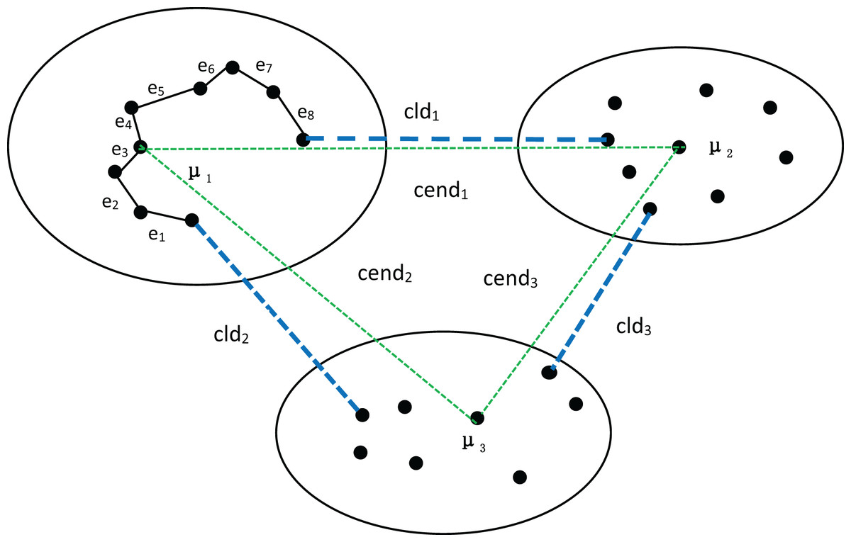
Figure 1: Three clusters, with density peaks , and being the center points of the three clusters.
The distances between the density peaks are , and . The distances between the three clusters are , and . In the cluster with as the center point, the minimum distance of each object is , , , etc.
Many algorithms use the average value of all data objects in a cluster as the center point to measure the degree of separation between clusters. While the average value can effectively represent a cluster in spherical datasets, it performs poorly for ring, semi-ring, and flow-shaped datasets. Because the object obtained by averaging is not within the cluster and is not a real data point, using it to measure inter-cluster separation can lead to inaccurate or erroneous results. To achieve a more balanced measure of inter-cluster separation, we utilize density peaks for calculation, as they represent real data points with high density. However, when the distance between clusters is very small, there is a high likelihood of a cluster being incorrectly split into two. Therefore, the minimum distance between clusters also significantly impacts the measurement of inter-cluster separation. Consequently, we employ sd to calculate the degree of separation between clusters.
To further validate the effectiveness of our method, we divided the dataset in Fig. 1 into four clusters, as shown in Fig. 2. We can observe that both the distance between density peaks ( ) and the minimum distance between clusters ( ) have suddenly decreased, while the compactness within the clusters remains almost unchanged. At this point, the average compactness within the clusters is similar to the value of , indicating that the denominator of MPV Formulation has not changed significantly. However, the numerator suddenly shrank, resulting in a sharp decline in the MPV (Minimum Distance and Peak Variation). Therefore, the number of clusters is 3, not 4.
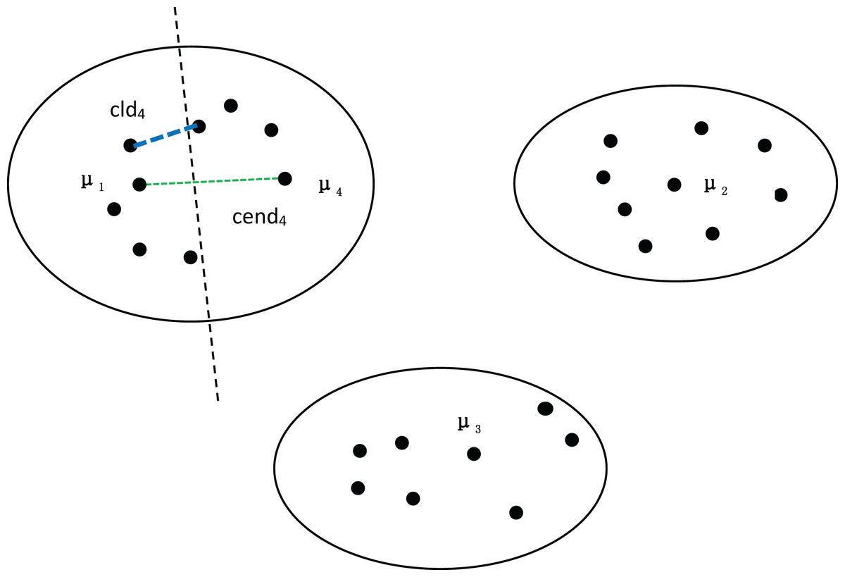
Figure 2: Four clusters, with density peaks of , , and .
The distance between the first-density peak and the fourth-density peak is cend4, and the distance between the first cluster and the fourth cluster is .
Next, we discuss the ring dataset and verify the effectiveness of our algorithm. At the same time, MPV performs well on ring, semi-ring, and flow-shaped datasets because it does not calculate the distance between all points and a center point when assessing cluster compactness. Instead, MPV starts from a point and identifies the closest neighboring point within the cluster. The distance to this nearest neighbor is recorded as the minimum distance from other points. In Fig. 3, there are two clusters, β and α. If is the center point of the cluster α, to calculate the distance from A to the compactness within the cluster cannot be expressed well. However, calculating the distance from A to B effectively indicates whether the cluster is compact. Additionally, the distance from A to C is much larger than that from A to B, which helps avoid misassigning point C to cluster α.
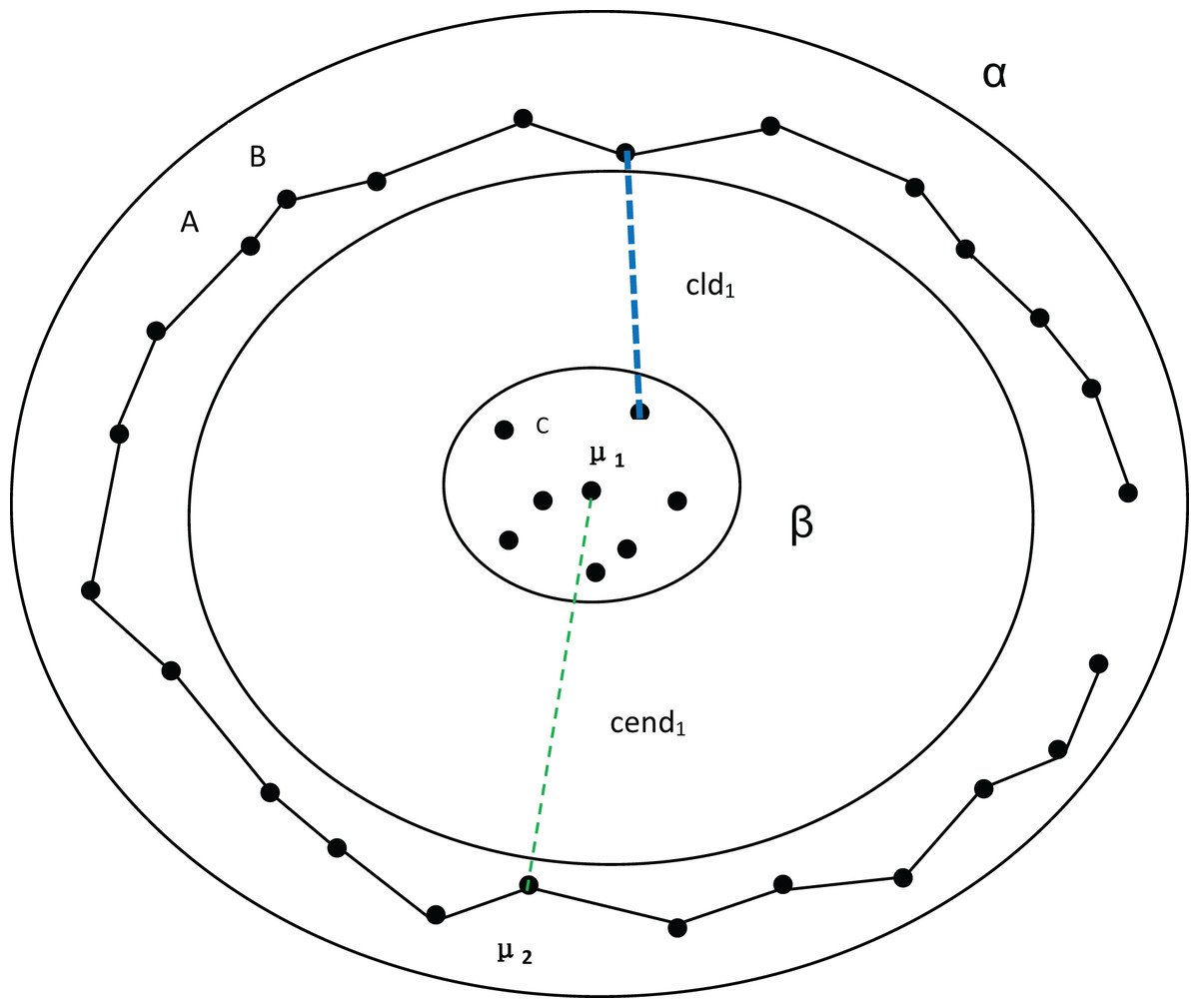
Figure 3: Two clusters, α and β.
Among them, A and B belong to cluster α. C belongs to cluster β. represents the distance between density peaks and , while represents the minimum distance between the two clusters.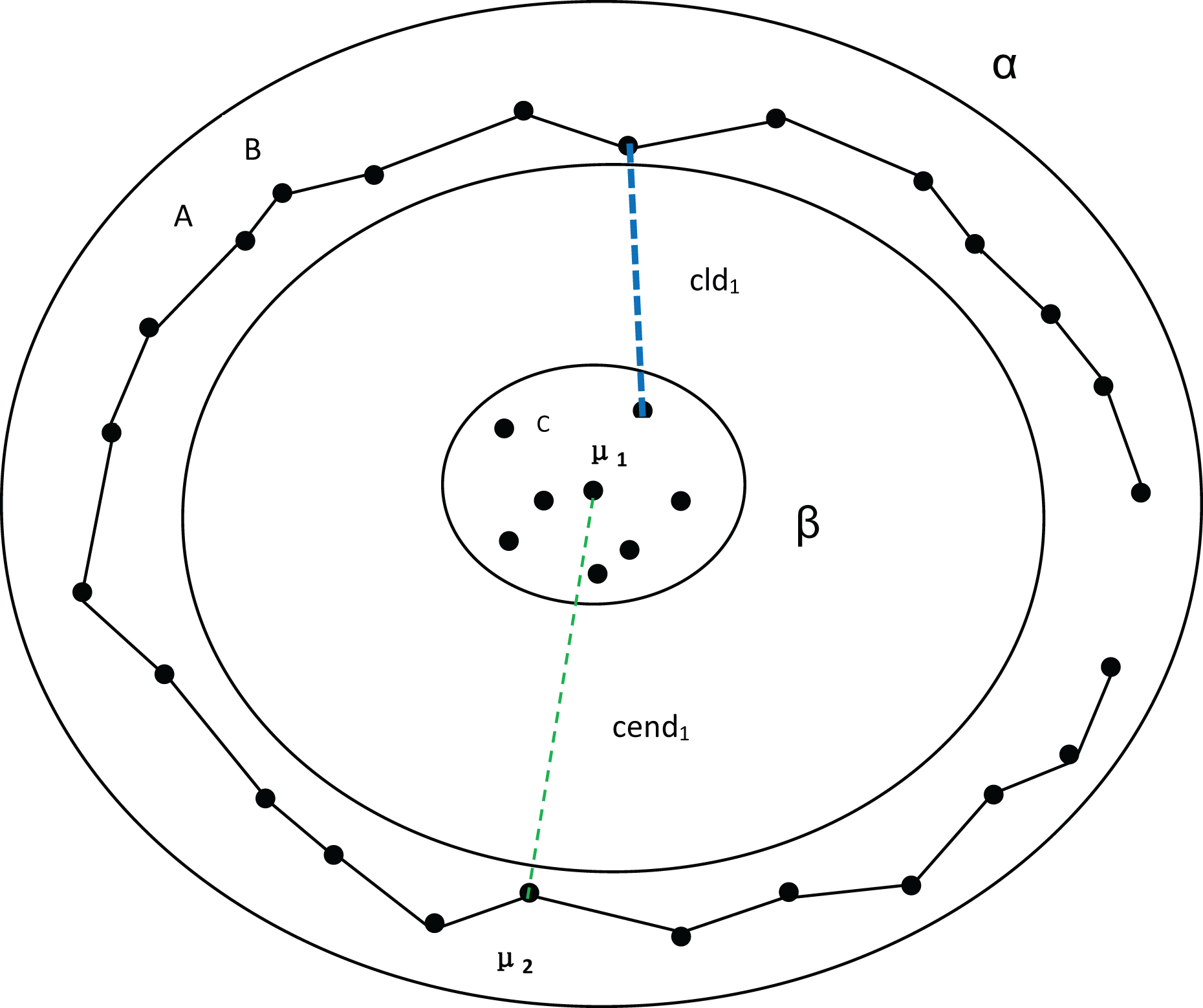
In Fig. 4, assuming that cluster α in Fig. 3 is divided into two clusters, we can observe that there are no significant changes in the compactness within the clusters or the values between density peaks. However, the inter-cluster distance suddenly decreases, which also causes a sudden drop in MPV. Consequently, the optimal number of clusters is determined to be 2 instead of 3.
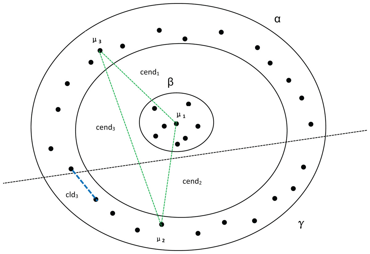
Figure 4: Three clusters, with α being divided into two clusters.
, and represent the distances between the three density peaks, respectively, and represents the minimum distance between cluster α and cluster γ.
Through the above arguments, we can see that MPV has a good effect on determining the number of clusters in the data.
Time complexity analysis
Assume that the data set has n objects and is divided into clusters. The time complexity for calculating is . The time complexity of calculating is . When computing the compactness within clusters, the time complexity is , derived from the series . Consequently, the overall time complexity of MPV is .
Use MPV to determine the best cluster number
In order to better reflect the intra-cluster compactness of all clusters, we select the maximum value of all intra-cluster compactness as the intra-cluster compactness of the dataset. MPV is a k-determination method that identifies the optimal by detecting the largest change in the separation measure . For the data set Parabolic5, the selection process of the best cluster number is shown in Fig. 5. Table 1 presents the detailed information of Parabolic5.
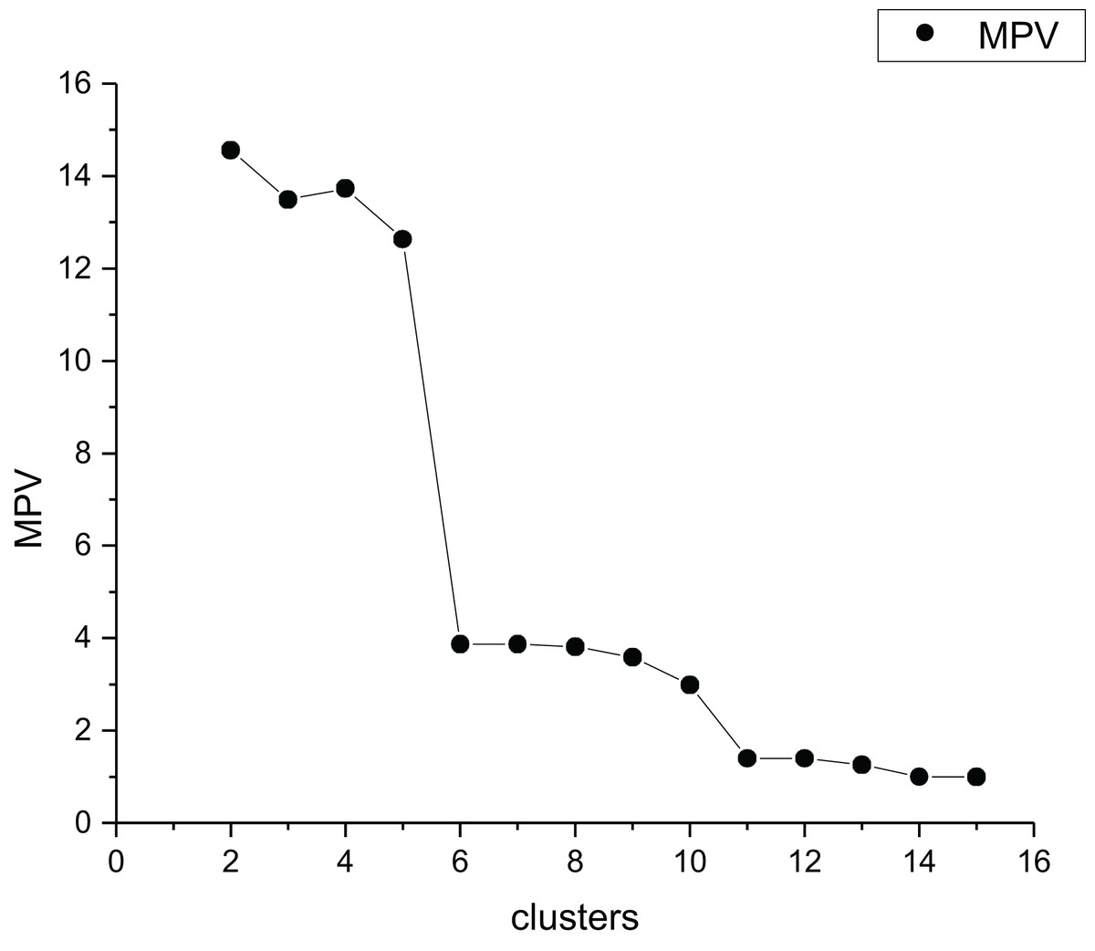
Figure 5: The MPV index change graph for different cluster quantities of Parabolic5.
| Number | Dataset | Dimension | Cluster number | The number of instances |
|---|---|---|---|---|
| 1 | R2 | 2 | 2 | 1,102 |
| 2 | R4 | 2 | 4 | 1,626 |
| 3 | R3 | 2 | 3 | 1,100 |
| 4 | Ringcirl3 | 2 | 3 | 1,500 |
| 5 | Ring4 | 2 | 2 | 1,233 |
| 6 | Parabolic2 | 2 | 2 | 1,000 |
| 7 | Parabolic3 | 2 | 3 | 1,500 |
| 8 | Parabolic5 | 2 | 5 | 2,500 |
| 9 | Segment 7 | 2 | 7 | 3,500 |
| 10 | Segment 11 | 2 | 11 | 5,500 |
| 11 | Spiral | 2 | 3 | 312 |
| 12 | Flame | 2 | 2 | 240 |
| 13 | S1 | 2 | 15 | 5,000 |
| 14 | S2 | 2 | 15 | 5,000 |
| 15 | S3 | 2 | 15 | 5,000 |
| 16 | S4 | 2 | 15 | 5,000 |
| 17 | A1 | 2 | 20 | 3,000 |
| 18 | A2 | 2 | 35 | 5,250 |
| 19 | A3 | 2 | 50 | 7,500 |
| 20 | Unbalance | 2 | 8 | 6,500 |
| 21 | Madelon | 500 | 2 | 4,400 |
| 22 | Banknote | 4 | 2 | 1,372 |
| 23 | Cardiocagraphy | 21 | 3 | 2,126 |
| 24 | Heart | 13 | 2 | 303 |
| 25 | Iris | 4 | 3 | 150 |
| 26 | Raisin | 7 | 2 | 900 |
| 27 | Seeds | 7 | 3 | 210 |
| 28 | DIM32 | 32 | 16 | 1,024 |
The formula for calculating the number of clusters is as follows:
Here, represents the cluster number, represents the maximum value of the search range, and represents the optimal cluster number.
Experimental studies
In this chapter, the k-determination method proposed in this article is validated on both artificial and real-world datasets to verify its practicality and effectiveness. In the experiment, our method is compared with over ten other significant methods, including CH, BIC, Dunn, Silhouette, etc. To ensure a fair comparison across the 14 algorithms, the density peak clustering algorithm (DPC) is employed as the underlying method.
Specifically, our method and the other typical methods are based on the density peak clustering algorithm to determine the cluster number. Detailed information regarding the typical algorithms for cluster number determination and the proposed method in this article is presented in Table 2.
| Number | Methods | Criteria for selecting K | Minimum number of clusters |
|---|---|---|---|
| 1 | Partition coefficient (PC) (Bezdek, 1973) | Maximum value | 2 |
| 2 | Zhao Xu Fränti (ZXF) index (Zhao, Xu & Fränti, 2009) | Knee | 2 |
| 3 | Last leap (LL) (Gupta, Datta & Das, 2018) | Maximum value & 1 | 1 |
| 4 | Last major leap (LML) (Gupta, Datta & Das, 2018) | Maximum value & 1 | 1 |
| 5 | Bayesian information criterion (BIC) | Maximum value | 2 |
| 6 | I index (Maulik & Bandyopadhyay, 2002) | Maximum value | 2 |
| 7 | Caliński Harabasz (CH) index (Caliński & Harabasz, 1974) | Maximum value | 2 |
| 8 | Classification entropy (CE) (Bezdek, 1975) | Minimum value | 2 |
| 9 | Fuzzy hypervolume (FHV) (Dave, 1996) | Maximum value | 1 |
| 10 | Dunn index (Dunn, 1973) | Maximum value | 2 |
| 11 | Silhouette index (Fujita, Takahashi & Patriota, 2014) | Maximum value | 2 |
| 12 | CVDD (Hu & Zhong, 2019) | Maximum value | 2 |
| 13 | WB index (Zhao & Fränti, 2014) | Minimum value | 2 |
| 14 | Our approach | Maximum value & 2 | 2 |
To compare the k-detection accuracy of 13 baseline methods and MPV on ring, semi-ring, flow-shaped, and spherical datasets, we conducted experiments on 28 datasets. The two-dimensional distribution structures of the synthetic datasets are shown in Figs. 6–10. Among these datasets, R2, R4, R3, ringcirl3, and Ring4 are ring and semi-ring datasets; Parabolic2, Parabolic3, Parabolic5, segment7, segment11, Spiral, and flame are flow-shaped datasets; S1–S4, A1–A3, and Unbalance are spherical datasets. Madelon is a high-dimensional artificial dataset with a dimensionality of 500. The real-world datasets used are Banknote, Cardiocagraphy, Heart, Iris, Raisin, Seeds, and Dim32. Table 1 presents the detailed information of all the datasets.
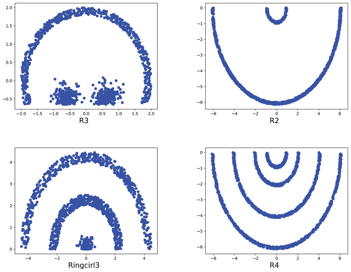
Figure 6: The two-dimensional structure diagram of the artificial datasets (R3, R2, Ringcirl3, R4).
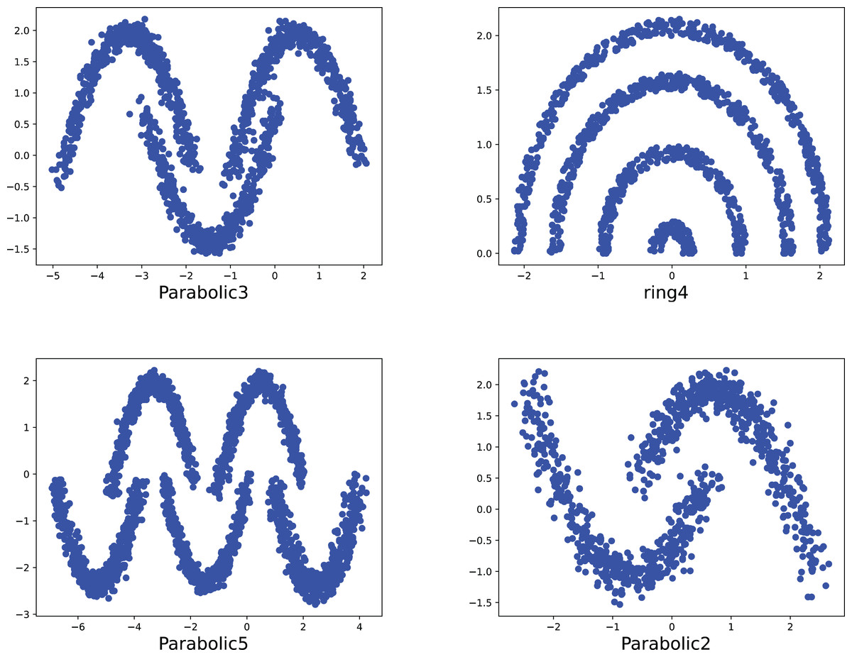
Figure 7: The two-dimensional structure diagram of the artificial datasets (Parabolic3, Ring4, Parabolic5, Parabolic2).
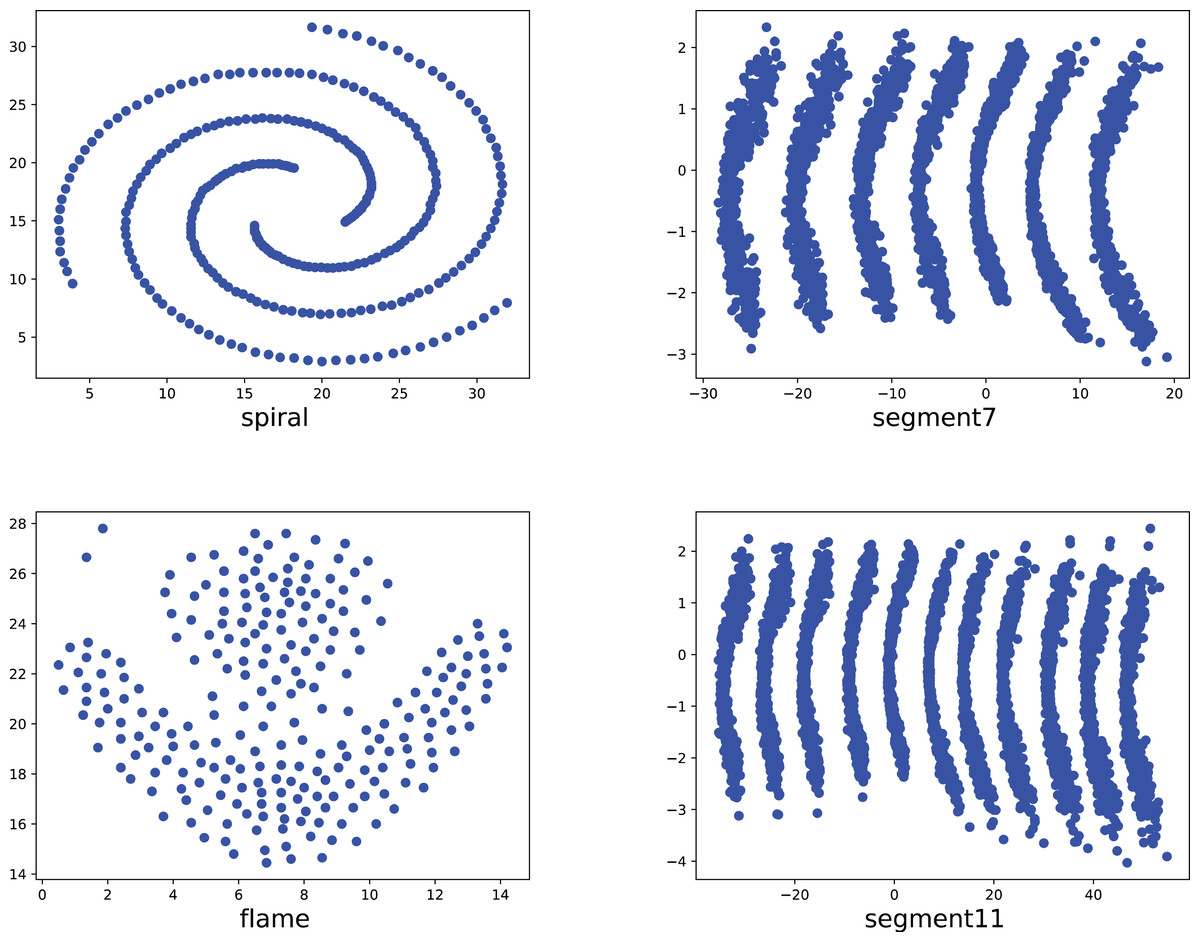
Figure 8: The two-dimensional structure diagram of the artificial datasets (Spiral, Segment7, Flame, Segment11).
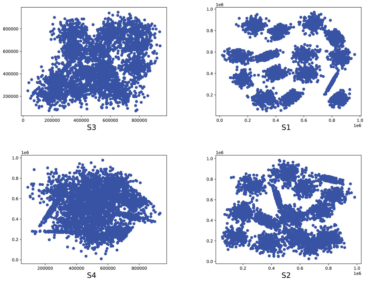
Figure 9: The two-dimensional structure diagram of the artificial datasets (S3, S1, S4, S2).
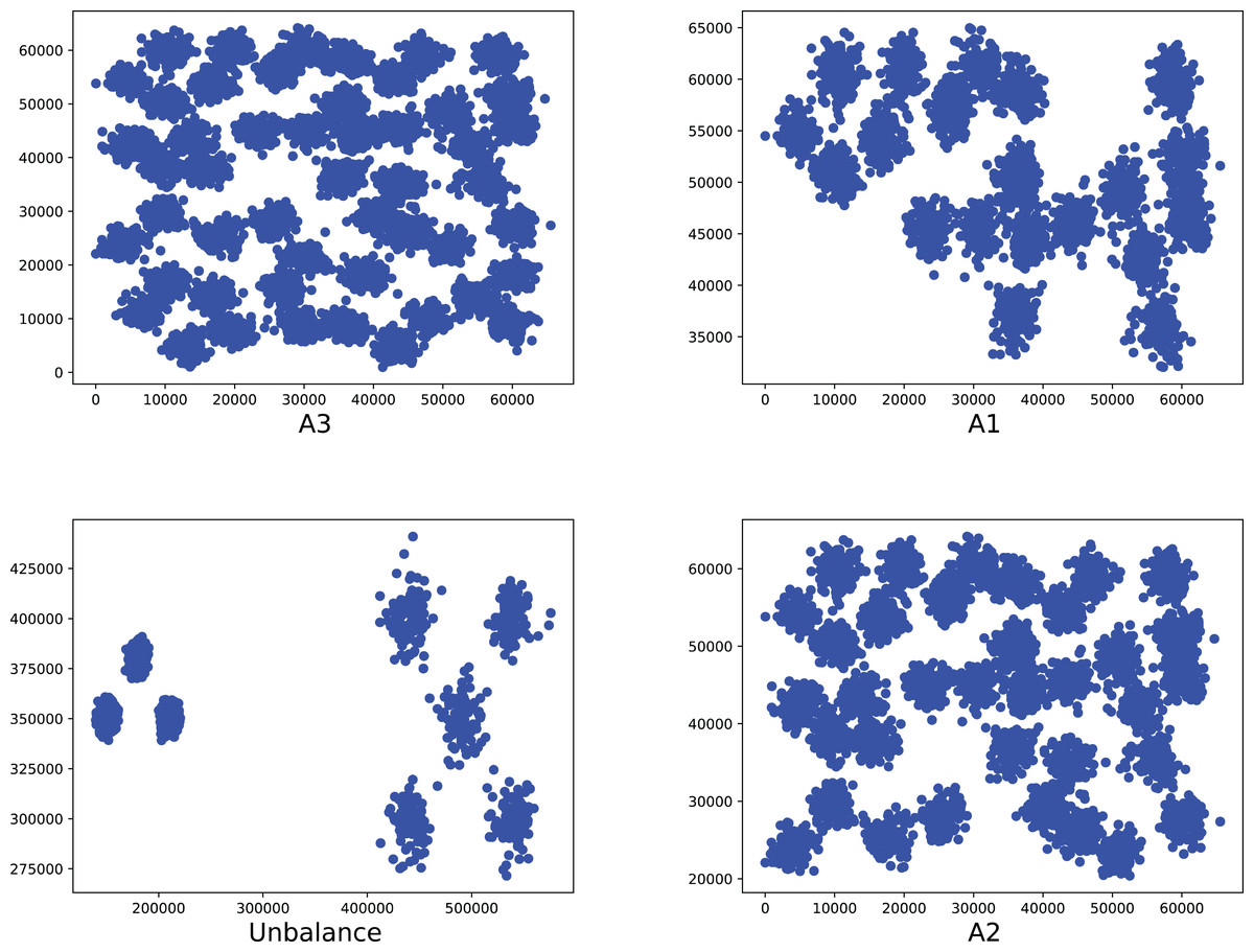
Figure 10: The two-dimensional structure diagram of the artificial datasets (A3, A1, Unbalance, A2).
Discussion
Experimental discussion on ring, semi-ring, and flow shape datasets
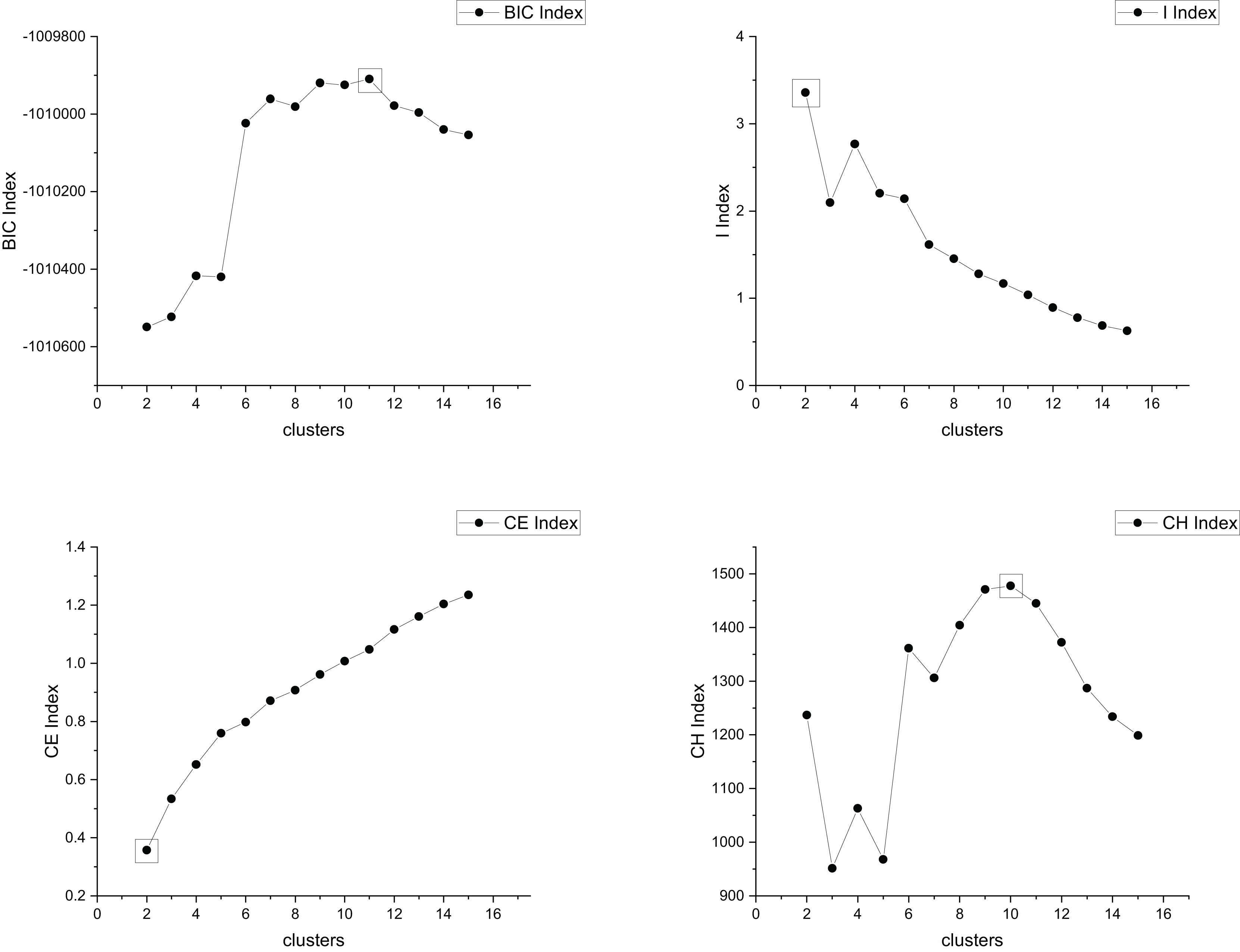
The true cluster number for the Parabolic2 dataset is 2. The results of the 14 methods used for obtaining the cluster number of Parabolic2 are shown in Figs. 11–14. From these figures, we can see that PC, I, CE, Dunn, CVDD, and our proposed method correctly identify the cluster number as 2. In contrast, the other seven methods fail to determine the correct cluster number. Specifically, ZXF yields a cluster number of 8; LL results in 3; LML and BIC both give 11; CH produces 10; Sil returns 6; and WB also indicates 10. The results from these methods are all incorrect.
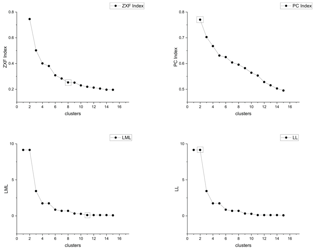
Figure 11: The relationship between approaches (ZXF index, PC index, LML, LL) and the number of clusters of Parabolic2.
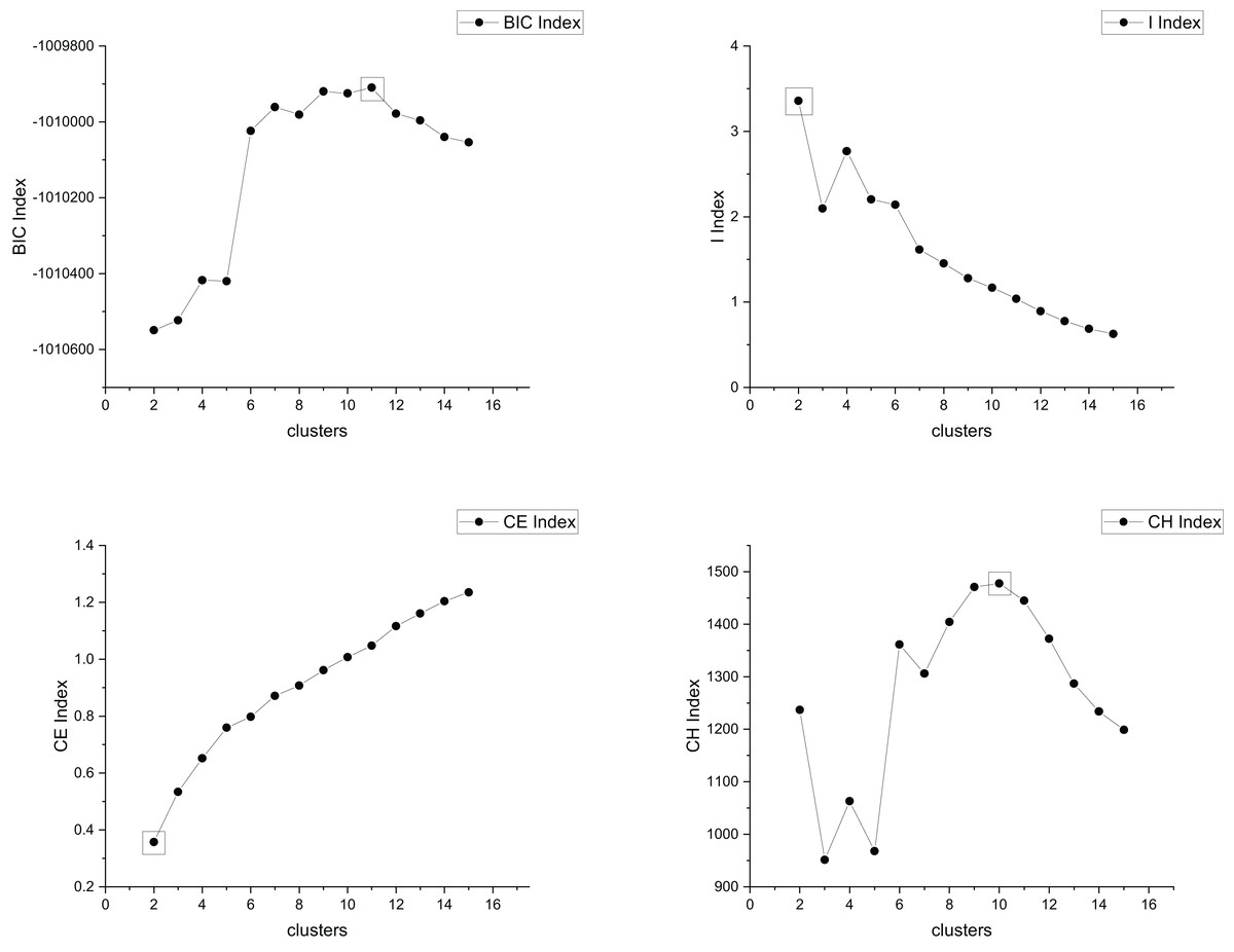
Figure 12: The relationship between approaches (BIC index, I index, CE index, CH index) and the number of clusters of Parabolic2.
Figure 13: The relationship between approaches (Dunn index, FHV index, CVDD index, Sil index) and the number of clusters of Parabolic2.
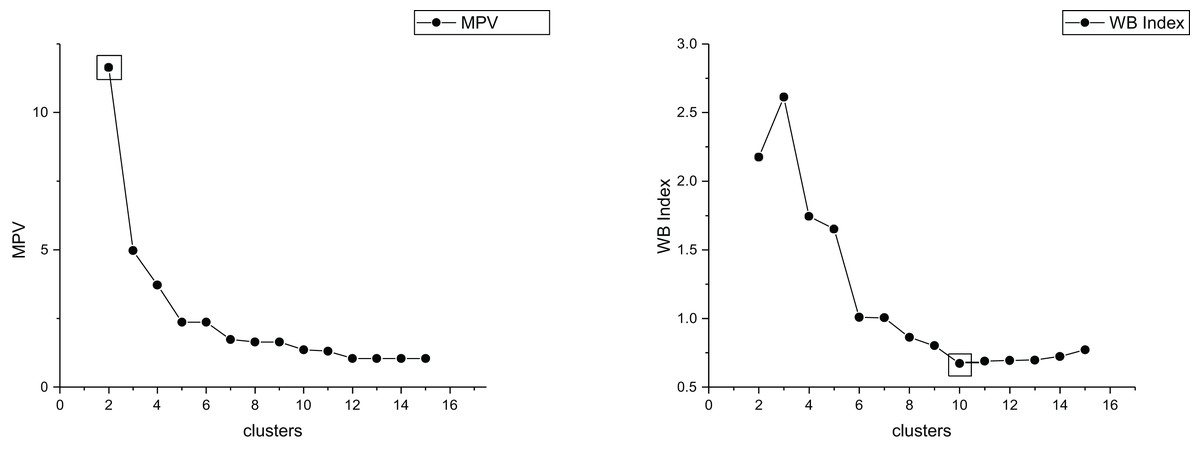
Figure 14: The relationship between approaches (MPV, WB index) and the number of clusters of Parabolic2.
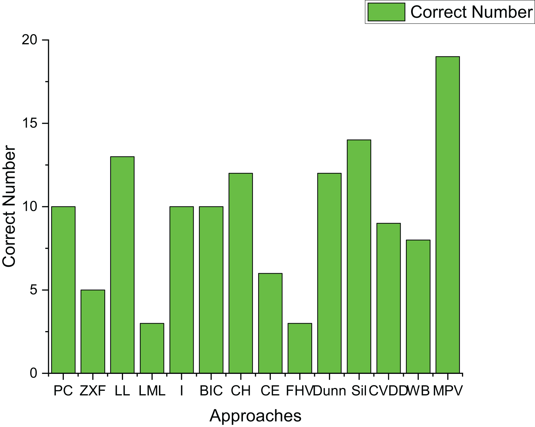
Table 3 presents the experimental results on 21 artificial datasets, including spherical datasets such as S1–S4, A1–A3, and Unbalance. Figure 15 shows how many datasets each algorithm correctly determined the number of clusters for. FHV performs poorly, only identifying the correct number of clusters for three datasets with clear boundaries and minimal noise, which indicates its noise sensitivity.
| Methods | R2 | R4 | R3 | Ringcirl3 | Ring4 | Parabolic2 | Parabolic3 | Parabolic5 | segment 7 | segment 11 | Spiral | flame |
|---|---|---|---|---|---|---|---|---|---|---|---|---|
| PC | 2 | 2 | 2 | 2 | 2 | 2 | 2 | 5 | 7 | 11 | 2 | 2 |
| ZXF | 9 | 7 | 7 | 16 | 13 | 8 | 11 | 5 | 7 | 8 | 6 | 3 |
| LL | 2 | 3 | 26 | 4 | 4 | 3 | 3 | 5 | 11 | 31 | 14 | 7 |
| LML | 18 | 8 | 26 | 7 | 8 | 11 | 20 | 20 | 11 | 39 | 14 | 7 |
| I | 2 | 3 | 7 | 3 | 4 | 2 | 2 | 5 | 7 | 11 | 6 | 2 |
| BIC | 2 | 2 | 33 | 2 | 2 | 11 | 35 | 43 | 7 | 54 | 2 | 2 |
| CH | 2 | 3 | 33 | 3 | 13 | 10 | 35 | 43 | 7 | 54 | 14 | 2 |
| CE | 2 | 2 | 2 | 2 | 2 | 2 | 2 | 2 | 2 | 11 | 2 | 2 |
| FHV | 1 | 1 | 1 | 2 | 1 | 1 | 1 | 1 | 7 | 11 | 1 | 1 |
| Dunn | 2 | 2 | 2 | 2 | 2 | 2 | 3 | 5 | 7 | 11 | 2 | 5 |
| Sil | 3 | 37 | 9 | 17 | 30 | 6 | 3 | 5 | 7 | 11 | 14 | 2 |
| CVDD | 2 | 2 | 3 | 3 | 3 | 2 | 21 | 5 | 7 | 11 | 17 | 3 |
| WB | 5 | 11 | 33 | 30 | 29 | 10 | 31 | 43 | 37 | 55 | 14 | 5 |
| Our method | 2 | 4 | 3 | 3 | 4 | 2 | 3 | 5 | 7 | 11 | 3 | 2 |
| Methods | S1 | S2 | S3 | S4 | A1 | A2 | A3 | Unbalance | Madelon |
|---|---|---|---|---|---|---|---|---|---|
| PC | 15 | 15 | 2 | 2 | 2 | 2 | 2 | 8 | 2 |
| ZXF | 15 | 15 | 15 | 14 | 13 | 15 | 12 | 5 | 16 |
| LL | 15 | 15 | 15 | 15 | 20 | 35 | 50 | 8 | 1 |
| LML | 28 | 22 | 27 | 21 | 20 | 35 | 50 | 21 | 1 |
| I | 2 | 3 | 2 | 2 | 3 | 3 | 3 | 8 | 2 |
| BIC | 15 | 15 | 15 | 2 | 20 | 35 | 50 | 8 | 19 |
| CH | 15 | 15 | 15 | 2 | 20 | 35 | 50 | 8 | 2 |
| CE | 2 | 2 | 2 | 2 | 2 | 2 | 2 | 8 | 2 |
| FHV | 1 | 1 | 1 | 1 | 1 | 1 | 1 | 8 | 1 |
| Dunn | 15 | 15 | 13 | 15 | 10 | 35 | 50 | 8 | 51 |
| Sil | 15 | 15 | 15 | 15 | 20 | 35 | 50 | 8 | 2 |
| CVDD | 15 | 14 | 17 | 9 | 16 | 34 | 36 | 8 | 3 |
| WB | 15 | 15 | 15 | 15 | 20 | 35 | 50 | 8 | 3 |
| our method | 15 | 15 | 15 | 2 | 20 | 35 | 50 | 3 | 2 |

Figure 15: The number of correctly estimated clusters for 21 artificial datasets by each method.
LL, CH, and Dunn show better performance, correctly determining the number of clusters for over ten datasets. However, their effectiveness is mainly limited to spherical datasets, where they achieve an 87.5% accuracy rate. In contrast, their performance on ring-shaped and complex-shaped datasets is less ideal.
Sil and WB also perform well on spherical datasets, achieving a 100% accuracy rate. Yet, their performance on ring-shaped and complex-shaped datasets is not as satisfactory, with the highest accuracy rate peaking at 50%.
To further verify the robustness of MPV in scenarios unfavorable to density measurement, this section supplements the analysis of two types of typical complex datasets: the high-dimensional sparse dataset (Madelon, 500 dimensions) and the density-differentiated dataset (Unbalance).
1. High-dimensional sparse scenario (Madelon dataset): High-dimensional data often causes the failure of distance measurement in traditional distance-based or density-related internal validity indices due to the “curse of dimensionality” (e.g., Euclidean distance cannot distinguish inter-cluster differences). As shown in Table 3, MPV correctly identifies the optimal cluster number k = 2 for this dataset, while the Dunn index (a traditional distance-based index) and CVDD (a density-involved distance index) misjudge it as k = 51 and k = 3, respectively. This advantage stems from MPV’s design: it constructs the separation degree sd using “density peaks (real data points) + minimum inter-cluster distances”, replacing the “virtual centroid distance” relied on by traditional indices and avoiding the problem of centroids deviating from real cluster structures in high-dimensional spaces.
2. Density-differentiated scenario (Unbalance dataset): This dataset contains “low-density large clusters + high-density small clusters” (as shown in Table 1, the sample size is 6,500, and the real k = 8). Traditional methods tend to misclassify low-density clusters as noise due to the global density threshold. Experimental results show that MPV accurately identifies k = 8, while FHV misjudges it as k = 1 and LML as k = 21. This benefit comes from MPV’s “sd/cd dynamic balance mechanism”: when there is a large density difference between clusters, cd (compactness) captures the loose characteristics of low-density clusters through the “maximum intra-cluster average of minimum distances”, preventing sd (separation degree) from being over-amplified due to local high-density peaks. Thus, robust cluster number determination is achieved in density-differentiated scenarios.
The above results indicate that MPV can still maintain higher accuracy than traditional methods in high-dimensional and density-differentiated scenarios (which are unfavorable to density measurement), verifying that it is not only applicable to density-uniform scenarios such as ring and semi-ring datasets.
The proposed method in this article demonstrates excellent performance, correctly determining the number of clusters for 19 out of 21 datasets. It is particularly effective for ring-shaped datasets and achieves a 75% accuracy rate for spherical datasets.
Experimental discussion on real-world datasets
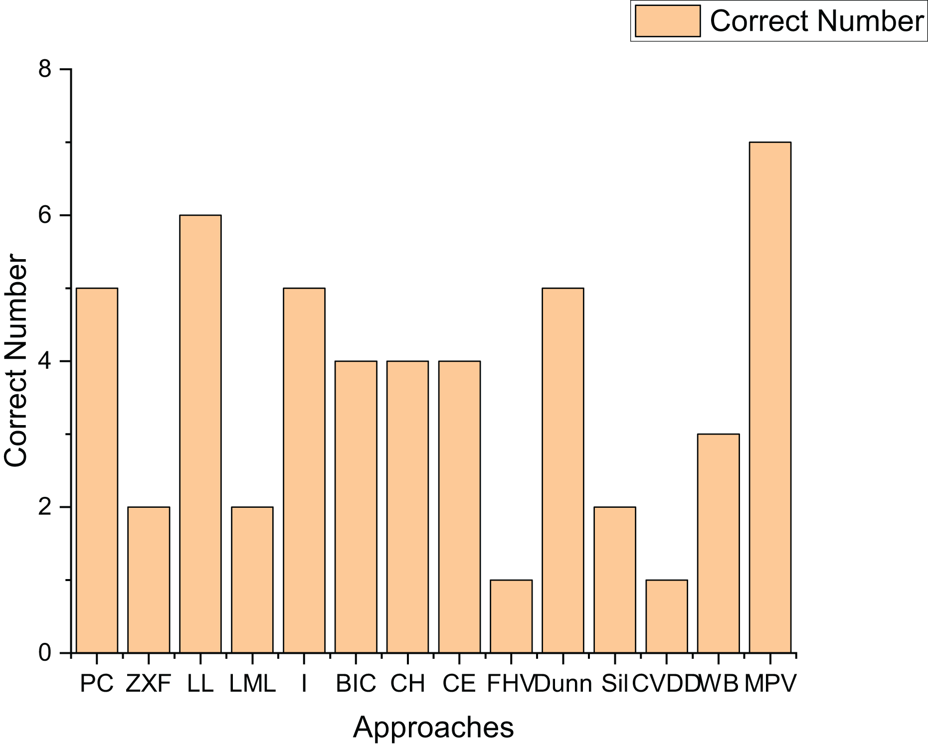
To further validate the effectiveness of our method, we applied 14 methods to estimate the cluster number on real-world datasets. Table 4 presents the experimental results on seven real-world datasets. Figure 16 shows the number of datasets for which each method correctly determined the number of clusters.
| Methods | Banknote | Cardiocagraphy | Heart | Iris | Raisin | Seeds | Dim32 |
|---|---|---|---|---|---|---|---|
| PC | 2 | 2 | 2 | 3 | 2 | 2 | 16 |
| ZXF | 14 | 7 | 6 | 3 | 5 | 4 | 16 |
| LL | 1 | 3 | 2 | 3 | 2 | 3 | 16 |
| LML | 1 | 3 | 10 | 5 | 20 | 5 | 16 |
| I | 2 | 3 | 2 | 3 | 5 | 2 | 16 |
| BIC | 2 | 13 | 2 | 8 | 23 | 3 | 16 |
| CH | 2 | 2 | 2 | 3 | 20 | 2 | 16 |
| CE | 2 | 2 | 2 | 12 | 2 | 14 | 16 |
| FHV | 1 | 1 | 1 | 1 | 1 | 2 | 16 |
| Dunn | 2 | 3 | 2 | 12 | 5 | 3 | 16 |
| Sil | 3 | 2 | 2 | 12 | 20 | 14 | 16 |
| CVDD | 37 | 2 | 17 | 2 | 29 | 2 | 16 |
| WB | 5 | 3 | 16 | 3 | 20 | 4 | 16 |
| Our method | 2 | 3 | 2 | 3 | 2 | 3 | 16 |
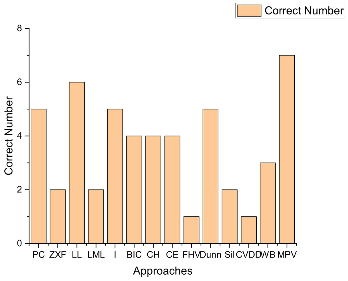
Figure 16: The number of correctly estimated clusters for real datasets by each method.
As indicated in Fig. 16, the performance of the Sil method on real-world datasets is inferior to that on artificial datasets. This is likely because the Sil method’s balance mechanism for compactness and separation is highly compatible with the geometric characteristics of spherical clusters, while real-world datasets often exhibit irregular structures. The PC, I, Dunn, and LL methods demonstrate relatively good performance on real-world datasets, correctly determining the number of clusters for at least five datasets. Notably, the method proposed in this article shows superior performance, accurately determining the number of clusters for all seven datasets. This fully proves the high effectiveness of the proposed method on real-world datasets.
Ablation study on MPV components
According to Table 5, we can draw the following experimental conclusions:
| Data | Component | ||
|---|---|---|---|
| sd only | cd only | sd + cd (MPV) | |
| Artificial datasets | 3 | 15 | 19 |
| Real-world datasets | 2 | 5 | 7 |
Limitations of single components
When relying solely on , among all 28 datasets (including 21 artificial datasets and seven real-world datasets), the number of clusters in only five datasets can be correctly identified. This indicates that relying solely on global separability cannot effectively capture the clustering characteristics of complex data structures, especially in non-convex datasets (such as circular and manifold datasets), where its performance is significantly limited.
When relying solely on , although the number of clusters in 20 datasets can be correctly identified (15 out of 21 artificial datasets and five out of seven real-world datasets), it has insufficient adaptability to non-spherical data (such as circular and manifold data). The local compactness metric is easily interfered with by complex boundaries, leading to problems of over-segmentation or under-segmentation.
Advantages of MPV
Among all 28 datasets, MPV can correctly identify the number of clusters in 25 datasets (19 out of 21 artificial datasets and seven out of seven real-world datasets), which significantly outperforms single components.
constrains global separability through the distance between density peaks, avoiding inter-cluster overlap (such as the linearly inseparable problem in the high-dimensional dataset Madelon). reinforces local compactness through the minimum intra-class distance, suppressing over-segmentation caused by noise (such as the continuous distribution characteristics of the circular dataset R2). The synergy between the two achieves robustness in complex scenarios.
MPV balances global separability and local compactness, addressing the inherent flaws of traditional single-index methods in complex data scenarios (such as excessive reliance on spherical assumptions and sensitivity to noise), and verifying the necessity of the two-component design.
Conclusions
In this article, we address the challenge of estimating the number of clusters in ring, semi-ring, and flow-shaped datasets. We propose MPV, a density-peak-based method for automated cluster number detection. By analyzing the change of the minimum intra-cluster distance and density peaks from a geometric perspective under varying k, MPV accurately identifies optimal cluster counts. Our method has been validated on ring, semi-ring, flow-shaped, and real-world datasets, demonstrating its practicality and effectiveness.