A novel transformer-based stacking ensemble method with multi-model integration for cancer classification
- Published
- Accepted
- Received
- Academic Editor
- Giovanni Angiulli
- Subject Areas
- Algorithms and Analysis of Algorithms, Artificial Intelligence, Data Mining and Machine Learning, Neural Networks
- Keywords
- Cancer classification, Machine learning, Transformer, Stack ensemble
- Copyright
- © 2025 Yang et al.
- Licence
- This is an open access article distributed under the terms of the Creative Commons Attribution License, which permits using, remixing, and building upon the work non-commercially, as long as it is properly attributed. For attribution, the original author(s), title, publication source (PeerJ Computer Science) and either DOI or URL of the article must be cited.
- Cite this article
- 2025. A novel transformer-based stacking ensemble method with multi-model integration for cancer classification. PeerJ Computer Science 11:e3314 https://doi.org/10.7717/peerj-cs.3314
Abstract
Background
Cancer classification using gene expression data presents significant challenges due to high dimensionality and complex biological patterns. While integrated learning approaches show promise, current methods often fail to capture complex model interactions and lack automated optimization frameworks.
Methods
We developed a novel hybrid machine learning framework combining traditional machine learning models with a Transformer-based stacked architecture for cancer classification. The framework employs a parallel optimization strategy for multiple base models (Random Forest, Gradient Boosting, eXtreme Gradient Boosting, and support vector machines) and utilizes a Transformer-based meta-learner for ensemble prediction. We evaluated the framework on a comprehensive cancer gene expression dataset containing 3,181 samples across five cancer types.
Results
The proposed framework achieved superior performance with over 99.7% accuracy across all cancer types. The Transformer-based meta-learner demonstrated particular effectiveness in handling complex cases, showing significant improvements in classification accuracy for rare cancer subtypes compared to traditional methods.
Discussion
Our hybrid framework successfully leverages the strengths of traditional machine learning algorithms and the advanced pattern recognition capabilities of Transformer architecture to provide a robust and interpretable solution for cancer classification. The research results indicate that this framework has potential application value in the fields of cancer diagnosis and model interpretability, marking an important advancement in the integration of learning technologies in the field of cancer classification.
Introduction
Recent global public health studies have shown a shift in epidemiologic patterns from communicable diseases to non-communicable diseases, the latter including different types of cancers. Worldwide, the incidence and prevalence of cancer is increasing in both developing and developed countries (Morhason-Bello et al., 2013; Olsen, 2015) Global cancer statistics estimate that in 2020 alone there will be about 19.3 million new cancer cases and nearly 10 million deaths from 36 types of cancer in 185 countries (Sung et al., 2021) According to projections, the cancer burden is expected to increase to 28.4 million cases by 2040 (Sung et al., 2021).
Cancer remains one of the leading causes of death worldwide, with millions of new cases diagnosed each year. The complexity and heterogeneity of cancer make effective diagnosis and treatment challenging. Early and accurate diagnosis is critical for selecting appropriate treatment strategies and improving patient prognosis. Recent advances in high-throughput gene expression profiling techniques have provided new insights into the molecular mechanisms underlying different cancer types (Lim et al., 2024). These datasets contain a wealth of information that can be used to develop predictive models for cancer classification.
Although traditional machine learning methods such as support vector machines, Random Forests (RFs), and logistic regression have demonstrated potential in gene expression data analysis and achieved acceptable performance in certain specific cancer classification tasks, these methods often fail to effectively capture the subtle interactions and complex nonlinear relationships between genes (Cruz & Wishart, 2007; Kourou et al., 2015). Traditional methods typically rely on manually designed feature engineering and domain expert knowledge to identify key biomarkers, a process that is not only time-consuming and labor-intensive but may also overlook important biological information (Guyon et al., 2002; Saeys, Inza & Larranaga, 2007). Additionally, traditional methods have significant limitations in handling multi-omics data integration, temporal gene expression changes, and considering gene regulatory network structures (Hasin, Seldin & Lusis, 2017).
Recent advancements in deep learning, particularly the emergence of the Transformer architecture (Vaswani et al., 2017), have provided new opportunities to address these challenges. The Transformer can dynamically learn the importance weights between features through self-attention mechanisms without predefining relationships between features, enabling it to successfully capture complex long-range dependencies and patterns in multiple fields such as natural language processing and computer vision (Dosovitskiy et al., 2020). In the biomedical field, researchers have begun exploring the application of the Transformer architecture to tasks such as protein sequence analysis, DNA sequence modeling, and gene expression data processing (Dosovitskiy et al., 2020; Ji et al., 2021). In particular, variant models like TabTransformer, designed for tabular data, offer new approaches for handling structured high-dimensional data like gene expression (Huang et al., 2020). These models can automatically learn complex interaction patterns between genes, potentially capturing biological mechanisms that traditional methods struggle to identify, opening up new possibilities for the accuracy and interpretability of cancer classification (Borisov et al., 2024; Way & Greene, 2018).
In this article, we introduce a novel hybrid framework that combines the benefits of traditional machine learning models with Transformer-based meta-learning. Our approach addresses several key challenges: (1) Optimal utilization of multiple machine learning algorithms. (2) Efficient parallel optimization of the underlying models. (3) Advanced feature interaction modeling through the Transformer architecture. (4) Achieved a transition from traditional black-box models to SHapley Additive exPlanations (SHAP) interpretable models and transparent decision-making processes, thereby making complex machine learning decision-making processes understandable.
Materials and methods
Computing infrastructure
The experiments are based on a high-performance platform and are submitted by Slurm. The specific configurations are, OS: CentOS Linux release 7.5.1804 (Core), Memory: 256 GB, Number of cores: 51.
The workflow
Base models (such as Random Forest, eXtreme Gradient Boosting (XGBoost), etc.) predict data and generate probability values. These probability values are fed into the Transformer, whose attention mechanism learns the relationships between the prediction results of different models. After multiple layers of processing, the final output is an optimized prediction result (Fig. 1). For example, if a particular base model performs exceptionally well on a specific type of sample, the Transformer will learn to assign a higher weight to that model’s prediction results when processing similar samples.
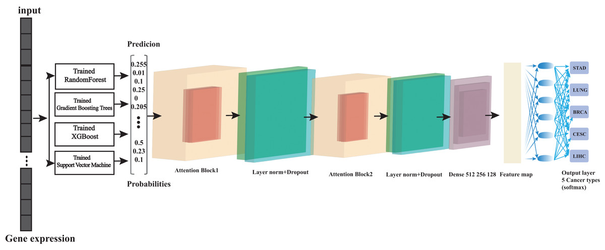
Figure 1: Overview of the architecture of ensemble learning system.
At its foundation, we have multiple base learners (Random Forest, Gradient Boosting, XGBoost, and support vector machine (SVM)) that operate in parallel, which is crucial for computational efficiency. Each base learner processes the input data and generates a probability matrix, where each row represents a sample and each column represents the probability of that sample belonging to a particular class. These probability matrices then serve as input to our Transformer meta-learner, which learns to combine these predictions optimally. The parallel training strategy significantly reduces computation time while maintaining model performance. This architecture effectively combines the strengths of traditional machine learning algorithms with the advanced pattern recognition capabilities of transformers.
Dataset
The Integrating Multiple Cancers dataset includes samples from different cancer types, each labeled with their respective cancer classification, all data is available at the following link, STAD: https://xenabrowser.net/datapages/?dataset=TCGA.STAD.sampleMap%2FHiSeqV2&host=https%3A%2F%2Ftcga.xenahubs.net&removeHub=https%3A%2F%2Fxena.treehouse.gi.ucsc.edu%3A443. LUNG: https://xenabrowser.net/datapages/?dataset=TCGA.LUNG.sampleMap%2FHiSeqV2&host=https%3A%2F%2Ftcga.xenahubs.net&removeHub=https%3A%2F%2Fxena.treehouse.gi.ucsc.edu%3A443. BRCA: https://xenabrowser.net/datapages/?dataset=TCGA.BRCA.sampleMap%2FHiSeqV2&host=https%3A%2F%2Ftcga.xenahubs.net&removeHub=https%3A%2F%2Fxena.treehouse.gi.ucsc.edu%3A443. CESC: https://xenabrowser.net/datapages/?dataset=TCGA.CESC.sampleMap%2FHiSeqV2&host=https%3A%2F%2Ftcga.xenahubs.net&removeHub=https%3A%2F%2Fxena.treehouse.gi.ucsc.edu%3A443. LIHC: https://xenabrowser.net/datapages/?dataset=TCGA.LIHC.sampleMap%2FHiSeqV2&host=https%3A%2F%2Ftcga.xenahubs.net&removeHub=https%3A%2F%2Fxena.treehouse.gi.ucsc.edu%3A443. (Table S1). The dataset contains expression levels of various genes across multiple cancer types. The initial dataset was preprocessed by removing any unnecessary columns and coding the categorical variables. Specifically, the “Cancer_tumor” column indicating cancer type was coded as a numeric value using LabelEncoder, Gene identifiers are gene symbols, such as BRCA1, TP53, EGFR, etc. For genome annotation versions, these cancer types (STAD, LUNG, BRCA, CESC, LIHC), the UCSC Xena Browser primarily uses GRCh37/hg19.
Data preprocessing
Although the use of gene expression data from the RNA-seq technique greatly facilitates the classification of cancers, it has its limitations due to the small sample size of a particular cancer type with a large number of genes (curse of dimensionality) (Blagus & Lusa, 2010; Yang & Naiman, 2014). In addition, the samples also contain genes that lack information which degrade the classification performance (García-Díaz et al., 2020; Vanitha, Devaraj & Venkatesulu, 2015), Therefore, before performing the analysis, it is necessary to preprocess the gene expression data.
To identify genes that were significantly differentially expressed in different cancer types, we performed analysis of variance (ANOVA) for each gene. After correction for the false discovery rate (FDR), genes with p-values <0.05 were considered differentially expressed and were selected for further analysis.
Data were preprocessed by removing non-informative columns such as sample identifiers and encoding categorical cancer type labels into numeric format using LabelEncoder. The matrix of Spearman correlation coefficients between samples was calculated by using the array-array strength correlation (AASI) method (Fig. 2), after which the average correlation coefficient between each sample and other samples was calculated, a threshold was set (the mean of the average correlation coefficients minus two times the standard deviation) from which potential outlier samples could be identified, and finally, samples of the filtered genes were normalized. Genes with low correlation were filtered out using the calculated threshold, returning genes with sample mean intensities greater than 0.809071442511119 (the mean of the mean correlation coefficient minus two times the standard deviation). In feature selection, a triple filtering mechanism was employed: variance filtering to remove genes with low variability, mutual information screening to retain genes associated with cancer, and correlation filtering to eliminate redundant genes (correlation coefficients > 0.96), ultimately retaining approximately 77% of the key genes. After preprocessing, the risk of dimensionality disaster is effectively reduced, thereby improving the generalization ability of the model.
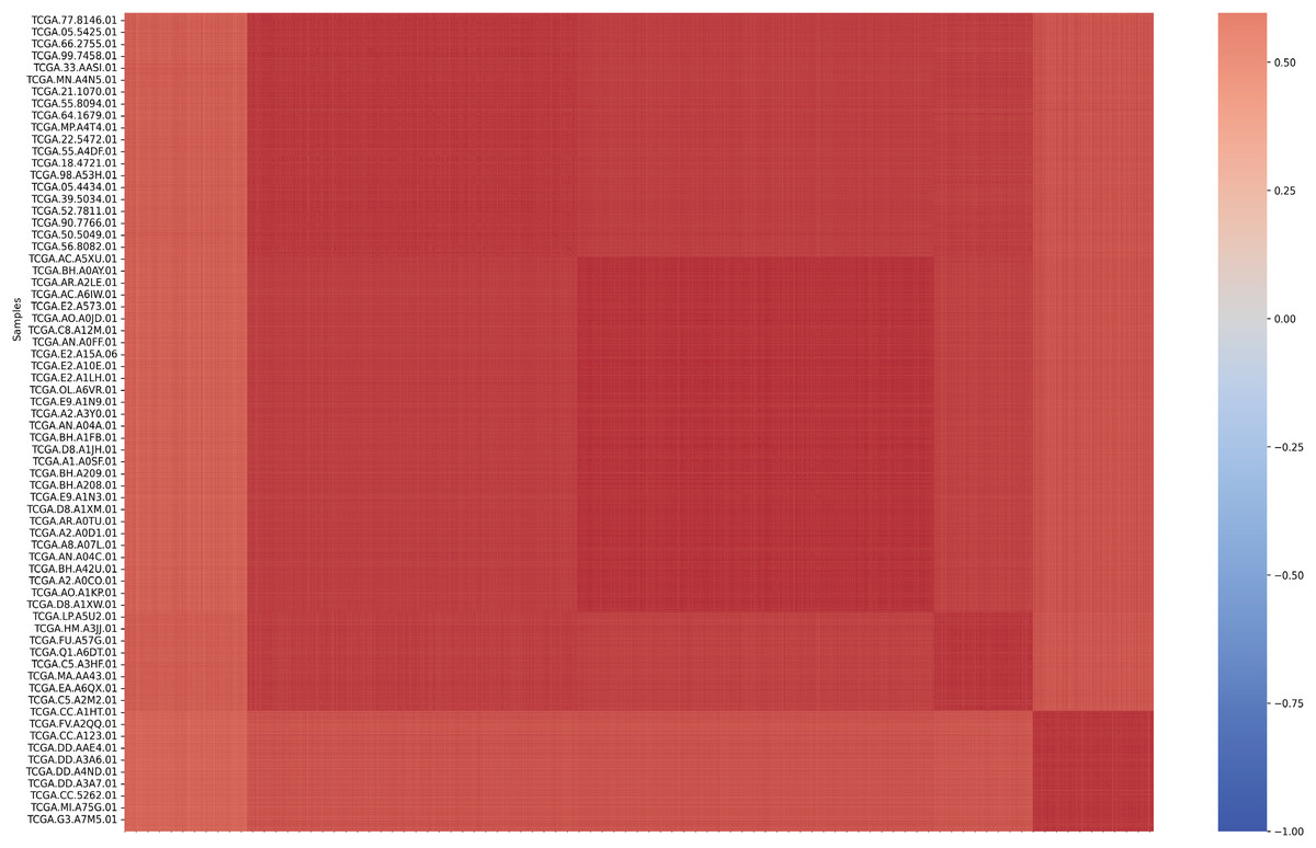
Figure 2: Array-Array Intensity correlation (AAIC) matrix defines the Pearson correlation coefficient between samples.
The matrix is usually displayed as a heat map, with each cell showing the correlation between two samples ranging from −1 (perfect negative correlation) to 1 (perfect positive correlation). This visualization is particularly valuable because it helps us understand the underlying structure of the data. The high correlation between samples of the same cancer type validates our feature selection, while the low correlation between samples of different cancer types shows that our features are effective in distinguishing between different types. The diagonal of this matrix shows perfect correlation (1.0), as it represents the correlation of each sample with itself.
Base model optimization
We evaluated multiple machine learning models, including RF (Breiman, 2001), Gradient Boosting (GBT) (Friedman, 2001), XGBoost (Chen & Guestrin, 2016), and support vector machine (SVM) (Shmilovici, 2023). Each model underwent extensive hyperparameter tuning using GridSearchCV to determine the optimal parameters. The models were trained and validated using an 80-20 training-test split, with the training data further split into training and validation sets (80-20) to prevent overfitting.
Our framework is based on four core models, each of which has been optimized for hyperparameters using parallel grid search combined with 10-fold cross-validation (Table S2). The optimization process utilizes ProcessPoolExecutor to achieve efficient computation across multiple CPU cores.
Cross-validation (Bates, Hastie & Tibshirani, 2024), also known as rotation estimation, is a model validation technique used to assess the quality of statistical analysis and results, with the goal of enabling the model to generalize to an independent test set (Fig. 3). During model deployment, differential validation is critical for evaluating the predictive accuracy of the model in real-world applications. During cross-validation, the model is typically trained using a dataset of known type.
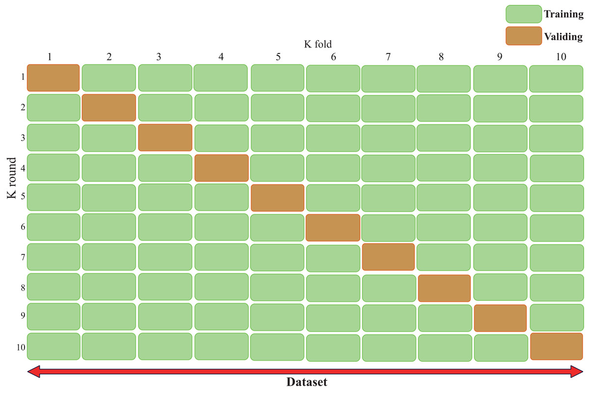
Figure 3: Cross validation technique demonstrating our validation strategy of dividing the dataset into five equal parts.
The figure shows that in each fold, nine parts are used for training and one part is used for validation. This process is repeated ten times and each part is used once as a validation set. This approach is crucial to ensure that our results are robust and generalizable. The figure typically shows the ten different colored sections and how they rotate between training and validation roles, helping the reader understand how we can maintain a consistent class distribution across all folds while ensuring that each sample is used for both training and validation.
In contrast, unknown-type data is used to test the model. This helps describe the features of the dataset used to test the model through the validation set during the training phase. There are two types of cross-validation: exhaustive cross-validation, including leave-one-out cross-validation (Rayo & Hoteit, 2012) and p-cross-validation (Liu, 2019); and non-exhaustive cross-validation, including K-fold cross-validation and repeated random subsampling cross-validation.
When using K-fold cross-validation, the entire training dataset can be divided into k disjoint folds, where each fold is a subset of the data used as the test set in one iteration, while the remaining k-1 folds are used as the training set. In each iteration, the model is trained on k-1 folds and tested on the remaining fold. The performance metrics for that iteration are recorded, and the entire cycle is repeated k times. After all iterations are completed, the average performance metrics across all iterations are calculated, and the optimal parameter combination is selected to obtain the optimized model.
Transformer-based meta-learning architecture
We propose an innovative stacked ensemble architecture based on Transformer meta-learning, which can dynamically integrate the prediction results of multiple base classifiers. Our method extends traditional stacked ensemble methods by replacing traditional simple meta-learners with attention-based deep neural networks, which can learn complex relationships between the prediction results of base models. Our ensemble foundation consists of four distinct base classifiers, selected based on their complementary strengths in different aspects of classification tasks. For example, the Random Forest Classifier (RFC) was chosen for its ability to capture nonlinear feature interactions and its robustness to outliers through bootstrap aggregation. For the meta-learners’ input, a clever transformation is applied: the prediction probabilities from all base models are reshaped into a sequence format. For example, when using four base models in a three-class classification problem, the input for each sample is a sequence of length 12 (4 models × 3 probabilities per category). The purpose of this operation is to make the data compatible with the Transformer’s input format, thereby leveraging the self-attention mechanism to learn relationships between prediction values. The meta-learners adopt a complex Transformer architecture, including: (1) Dual multi-head attention layers (eight heads per layer). (2) Layer normalization and Dropout for regularization. (3) Dense layers with gradually decreasing Dropout rates. (4) A Softmax output layer for final classification.
Input layer and feature representation
The meta-learner receives probabilistic predictions from all base models as input. For a classification problem with K classes and M base models, this creates an input matrix of dimension N × (K × M), where N is the number of samples. We reshape this input into a sequence format of dimension (N × 1 × (K × M)) for Transformer processing. This reshaping operation converts the flat probability vector into a format that can be processed by a self-attentive mechanism that treats each model’s prediction as a sequence element.
Multiple attention mechanisms
Two consecutive multi-head attention layers are used, each containing eight attention heads. Each attention head can be imagined as a specific angle of analytical perspective; the attention heads in the first layer may learn that some heads may focus on relationships between similar models (e.g., Random Forest and XGBoost), others may focus on relationships between complementary models, and still others may focus on identifying certain specific types of predictive patterns; the attention heads in the second layer build on the first layer with a more higher level of integration, may learn the reliability of different model combinations in different scenarios, identify the predictive advantages of certain models on specific categories, and discover complex predictive patterns across models.
Unlike traditional voting or simple weighting methods, this framework enables dynamically assign weights to each prediction. For example, if a prediction from a random forest is found to be particularly reliable in a certain situation, the system will automatically increase its influence. With deep neural networks, the system can learn complex integration methods that go far beyond simple weighting. It may discover patterns such as “pay special attention when both Model A and Model B are highly confident, but Model C holds the opposite opinion”. Instead of using fixed rules, the attention mechanism allows the system to adapt the integration strategy to the specifics of the current prediction. The architecture makes it easy to integrate new base models by simply adding the predictions of the new model to the input sequence.
Performance evaluation
To comprehensively assess the classification performance of our machine learning models, we employed multiple evaluation metrics that capture different aspects of model performance. The selection of these metrics is crucial for multi-class cancer classification, as it provides a holistic view of model effectiveness across different cancer types.
- 1.
Accuracy
Accuracy represents the proportion of correctly classified samples among all samples and serves as the primary metric for overall model performance:
(1) where: TP = true positives, TN = true negatives, FP = false positives, FN = false negatives.
For multi-class classification, accuracy is calculated as:
(2)
- 2.
Confusion matrix
The confusion matrix provides a detailed overview of the classification performance for each cancer type. For our multi-class problem (STAD, LUNG, BRCA, CESC, LIHC), the confusion matrix is a 5 × 5 table, where rows represent actual cancer types, columns represent predicted cancer types, diagonal elements represent correct classifications, and non-diagonal elements represent misclassifications. The confusion matrix can be used to identify which cancer types are classified most accurately, common misclassification patterns between different cancer types, and performance differences among classifications.
- 3.
Precision, recall, and F1-score
For each cancer type , we calculated:
Precision (positive predictive value):
(3)
Precision measures the proportion of samples predicted as cancer type i that are actually cancer type .
Recall (sensitivity or true positive rate):
(4)
Recall measures the proportion of actual cancer type samples that are correctly identified.
F1-score (harmonic mean of precision and recall):
(5)
For our cancer classification problem, Transformer stacks performed best across all metrics.
Results
Model performance
Stacking is performed and finally the accuracy of the original stacked model is obtained, after which the final probability value is obtained by five-fold cross-validation. Figure 4 shows the accuracy rates of all models (including individual models and ensemble models). By visually comparing the performance of different models, the best model can be quickly identified. The Transformer-based stacked ensemble model consistently outperforms individual base models in terms of accuracy. The Transformer stack achieves an accuracy rate of 0.997, outperforming all individual models. This model effectively combines the strengths of the base models to enhance predictive performance.
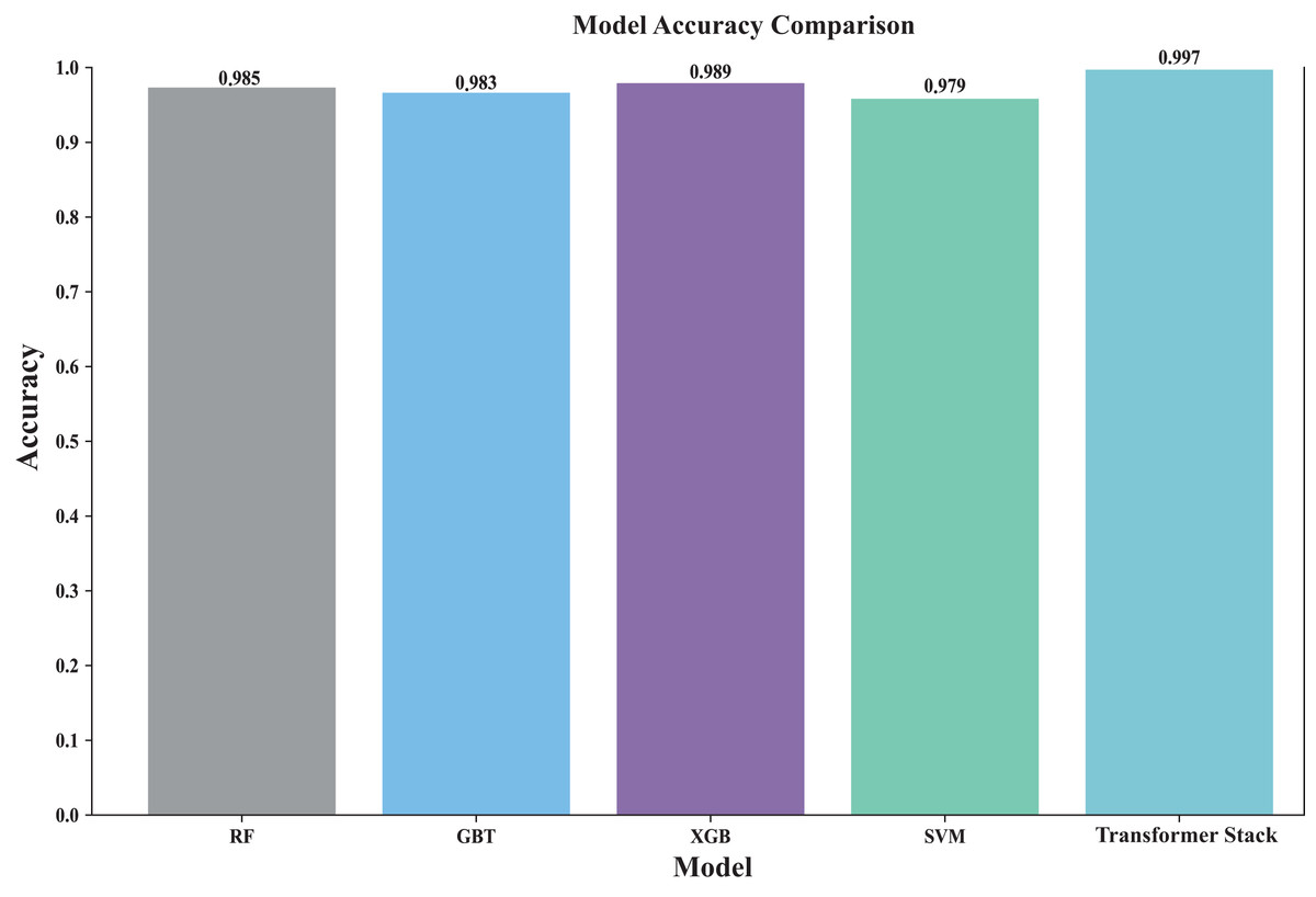
Figure 4: Comparison of the accuracy of each model.
This comparison plot shows the performance accuracy of each model in our ensemble, both the individual base learners and the converter-based ensemble. The figure uses bars to show the average accuracy across different cross-validation folds. This clearly shows how our ensemble approach outperforms individual models. It is particularly effective in showing the stability of predictions across different data splits and how the converter meta-learner successfully combines the strengths of each base learner.
Figure 5 shows the heatmap of the confusion matrix, illustrating the comparison between the model’s predictions on the test set and the actual labels. The model’s performance across each category is detailed, identifying which categories are prone to confusion, and through an in-depth analysis of the model’s classification performance, areas for improvement are identified. It can be seen that by stacking the classification and identification of the five types of cancer, the classification performance has significantly improved. Among them, the performance of individual models was the worst, and TabNet performed worse than the Transformer stack (precision: 0.9972) in terms of metrics (precision: 0.9723). In addition, we compared traditional stacking with Transformer stacking (Fig. S1). The results showed that the Transformer-based stacking method further improved classification accuracy. A Friedman test (multiple comparison) was performed, with a p-value <0.05, indicating statistical significance. This proves the necessity of integrating predictions based on Transformer machine learning models.
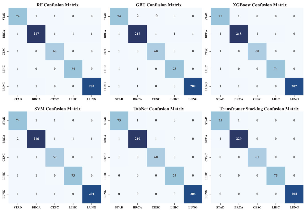
Figure 5: Heat map of confusion matrix.
The confusion matrix heatmap shows in detail the classification performance of our model in different cancer types. Each row represents the actual category and each column represents the predicted category. Darker colors usually indicate a higher number of predictions. It shows not only the overall accuracy, but also where misclassification occurs. It helps to determine whether certain cancer types are more likely to be confused with others, providing insight into potential areas of improvement as well as the strengths and limitations of the model with respect to specific cancer types.
Figure S2a illustrates how model training scores and cross-validation scores change with the number of training samples. This method can be used to determine whether the model suffers from overfitting or underfitting, and whether adding more training data can improve performance. It is necessary to decide whether to collect more data or adjust the model complexity. Observation of the results in Fig. S2b shows that when the batch size reaches 1,400 to 1,700, most models achieve good performance, and as the batch size increases, the standard deviation gradually decreases, indicating that the model stability has improved.
Table S3 shows the performance of each model during cross-validation. The average precision, recall and F1-score of the best model reached 0.9858, 0.9858 and 0.9858, respectively. while the classification accuracy was 98.58%. Moreover, these results after performing integration learning also show that our proposed model outperforms all individual models and machine learning results. In addition, Figs. 4 and 5 (confusion matrix) show that our proposed model has better classification performance compared to a single model.
SHAP analysis
We used SHAP analysis to identify 20 genes that are most important for cancer classification, meaning that these genes play a key role in model decision-making (Fig. S3a). SHAP (SHapley Additive exPlanations) values represent the marginal contribution of each gene to the final prediction result: the higher the value, the more significant the gene’s influence on classification decisions. SHAP values reflect how changes in gene expression drive model predictions toward specific cancer types. By interpreting the biological significance of important genes, we can better understand cancer changes (Fig. S3b). TSPY1 (SHAP: 0.0148)—Testis-specific protein Y-linked 1. This gene functions in cell proliferation and apoptosis regulation and is abnormally expressed in various tumors, particularly those of the reproductive system, making it a potential biomarker for gender-related cancers. NF525 (0.0126)—Zinc finger protein 525, this gene is a transcription regulator involved in gene expression regulation. The zinc finger protein family is closely associated with tumor suppression and carcinogenic processes. Its clinical significance lies in the fact that transcriptional regulation disorders are an important mechanism in cancer development. Additionally, SHAP analysis enhances model interpretability, enabling a transition from traditional black-box models to SHAP-explained models and transparent decision-making processes, thereby making complex machine learning decision processes understandable. We used functional classification heatmaps (Fig. S3c) and cancer association networks (Fig. S3d) to reveal how each gene influences cancer classification decisions, and used SHAP to quantify the magnitude and direction of gene contributions.
Model complementarity analysis
After analyzing the prediction patterns of different models, we found that they are significantly complementary. As shown in Fig. 5, although the models are similar in overall accuracy, the types of errors they make across the entire dataset are different. This complementarity is reflected in the low correlation between the error patterns of different underlying models, indicating that integrating their prediction results can produce better results.
Analysis of the attention model
An analysis of the attention weights of the Transformer architecture reveals interesting insights about how the model combines predictions: (1) First attention layer: the initial attention heads exhibit specialized behavior, with different heads focusing on different aspects of the base model predictions. We observe that certain heads are responsible for consistently focusing on high-confidence predictions, while others are responsible for focusing on cases where the base model is inconsistent. (2) Second attention layer: the secondary attention mechanism exhibits more context-dependent behavior, effectively weighting the fine-grained representations according to the specific characteristics of each input case. This layer shows particularly strong activation patterns for cases where the base model shows conflicting predictions.
Discussion
Since gene expression data contains a large number of genes, ordinary methods cannot utilize all of the gene information as features, and feature selection is often required to reduce the dimensionality of the dataset, but at the same time, some key information is lost. Therefore, in our study, we utilize parallel computing methods to improve computational efficiency, enabling us to retain most of the features (genes) containing information for classification and prediction.
The results of this study demonstrate the effectiveness of machine learning models in classifying cancer tumors based on gene expression data. The stacked ensemble model combining multiple classifiers achieved the highest accuracy, demonstrating that integrating different models can capture different aspects of the data and thus improve performance.
Our study emphasizes the importance of extensive hyperparameter tuning and model evaluation to determine the best performing model. Future work could explore additional machine learning techniques and larger, more diverse datasets to further improve classification performance.
Our stacked integrated model achieves higher classification accuracy across five cancer types (STAD, LUNG, BRCA, CESC, LIHC), building on the foundational research established in the field of cancer gene expression classification. Golub et al. (1999) first demonstrated the feasibility of using linear SVMs combined with microarray gene expression data for cancer classification, achieving 94% accuracy in leukemia classification using 7,129 gene features (only two errors out of 34 patients). Vapnik & Mukherjee (1999) subsequently improved accuracy to 100% using an enhanced weighted voting method. However, these early studies were limited to binary classification of a single cancer type and had relatively small sample sizes (38 training patients).
In contrast, our method targets multi-cancer classification across five distinct cancer types while handling significantly larger datasets and maintaining comprehensive feature retention. Unlike earlier SVM methods, our approach does not utilize all available features but instead addresses the computational complexity of high-dimensional data through parallel computation while retaining informative genes that traditional feature selection might discard. This marks a significant advancement from the binary classification paradigm established by Golub et al. (1999) toward more clinically relevant multi-class scenarios.
The Transformer attention mechanism reveals biologically meaningful patterns of gene importance. This interpretability is crucial for clinical acceptance, as it provides transparent reasoning for classification decisions. Multi-cancer classification capability can serve as a diagnostic aid, particularly for tumors of unknown primary origin. In addition, we used SHAP analysis to select 20 genes that reflect how gene expression changes drive model predictions toward specific cancer types, improving model interpretability, making complex machine learning decision processes understandable, clarifying the specific contribution of each gene to cancer classification, and providing a basis for classification decisions.
We also acknowledge the following limitations: (1) Reliance solely on TCGA data and lack of external validation limit generalizability to other populations and sequencing platforms; (2) lack of prospective clinical validation; (3) static classification methods do not account for the spatiotemporal dynamics of the disease. External validation using multi-institutional independent datasets should be prioritized. Integration with other omics data types and the development of uncertainty quantification methods will enhance clinical utility. The interpretability of the attention mechanism warrants further exploration to advance biomarker discovery and cancer biology research.
Conclusions
This study comprehensively evaluates various machine learning models for cancer tumor classification using gene expression data. The findings highlight the potential of ensemble learning and semi-supervised methods to improve prediction accuracy. These results contribute to the growing body of evidence supporting the use of machine learning in cancer diagnosis and have implications for personalized medicine and targeted therapies. In this work, we present a novel integrated architecture that successfully combines traditional machine learning models with Transformer-based meta-learning for cancer classification. The framework shows promising results in terms of both performance and computational efficiency. Five of the most common cancers that cause death in humans, namely stomach, lung, breast, cervical, and liver cancers, were classified using the RNA-seq gene expression dataset for each cancer tumor. Tumor classification using RNA-seq data is more accurate and usable than microarray data. We used the sample-wise Spearman correlation coefficient matrix calculated using mutual information and array-to-array strength correlation (AASI) methods as a feature selection method, and compared the performance of the proposed method with that of independent machine learning methods. The results showed that the proposed model achieved the highest performance compared to single machine learning methods. We conclude that our proposed model achieves the highest performance compared to single machine learning methods. Therefore, our proposed model can correctly classify all observed positive cancer cases. The model helps improve the detection and diagnosis of early cancer susceptibility, providing a basis for early intervention decisions to improve survival rates. Through SHAP interpretation, it makes complex machine learning decision-making processes understandable, clarifying the specific contribution of each gene to cancer classification, thereby providing a scientific basis for clinical applications.
Future work could explore the application of this approach to other complex biological classification tasks as well as the incorporation of other underlying models, should consider the potential impact of using many feature types, such as methylation and mutation, integrated with RNA-seq data, also consider improved stack integration issues, including statistical properties, to improve inference.
Supplemental Information
Comparison of different methods.
Traditional stacking methods, including hard voting (based on majority voting), soft voting (based on probability averaging), logistic regression stacking (using logistic regression as the meta-learner), and random forest stacking (using random forest as the meta-learner), are compared and discussed with the Transformer stacking method used in this study.
Learning rate curve and changes in training data across different batches.
a. The x-axis represents the number of training epochs, while the y-axis shows both training and validation metrics (typically loss and accuracy). This visualization is crucial for understanding the model’s learning dynamics, identifying potential overfitting, and validating the effectiveness of our learning rate schedule and early stopping criteria. The curve typically shows how the model’s performance improves over time and eventually stabilizes, demonstrating the effectiveness of our training strategy and the model’s convergence characteristics. b. Test batch sizes with finer granularity at 10%, 15%, 20%, 30%, 40%, 50%, 60%, 70%, 80%, 90%, and 100% to ensure sufficient data points to identify the inflection point of performance improvement.
SHAP analysis.
a. SHAP analysis identified 20 genes that are most important for cancer classification, meaning that these genes play a key role in the model’s decision-making process. b. By interpreting the biological significance of important genes through functional analysis, we can better understand cancer changes. c and d. Functional classification heat maps and cancer association networks reveal the impact of each gene on cancer classification decisions.
Number of samples in each class used in the classification.
Summary of downloaded data, including training and test scores for each cancer tumor.
Hyper-parameter optimized.
The foundation of our framework consists of four basic models, each of which is hyper-parameter optimized by a parallel grid search with cross-validation.
Performance of each model in cross-validation.
The performance of each model during cross-validation. The average precision, recall, and F1 score of the best model were 0.9858, 0.9858, and 0.9858, respectively, while the classification accuracy was 98.58%.