Exploring advanced techniques for enhancing CapsNet: custom squashing, pretraining, and routing in large-scale unbalanced data
- Published
- Accepted
- Received
- Academic Editor
- Giovanni Angiulli
- Subject Areas
- Artificial Intelligence, Data Mining and Machine Learning, Neural Networks
- Keywords
- GN-CapsNet, VGG-CapsNet, Capsule networks, Enhanced squash function, Modified dynamic routing, Fire-CapsNet, Unbalanced data
- Copyright
- © 2025 Al-Rahaawi and Aydın Atasoy
- Licence
- This is an open access article distributed under the terms of the Creative Commons Attribution License, which permits unrestricted use, distribution, reproduction and adaptation in any medium and for any purpose provided that it is properly attributed. For attribution, the original author(s), title, publication source (PeerJ Computer Science) and either DOI or URL of the article must be cited.
- Cite this article
- 2025. Exploring advanced techniques for enhancing CapsNet: custom squashing, pretraining, and routing in large-scale unbalanced data. PeerJ Computer Science 11:e3267 https://doi.org/10.7717/peerj-cs.3267
Abstract
Capsule networks (CapsNet) have emerged as a promising alternative to traditional convolutional neural networks (CNNs) for image classification, due to their ability to capture spatial hierarchies and relationships between parts and wholes. However, CapsNet still faces limitations such as high computational complexity, inefficient routing, and difficulty in learning complex features when trained from scratch. To address these issues, this study presents two enhanced methods to improve the performance of the baseline CapsNet model. The first method integrates pre-trained CapsNet architectures—including GoogLeNet-Inception V3-based CapsNet (GN-CapsNet), Visual Geometry Group-based CapsNet (VGG-CapsNet), and Residual Network-based CapsNet (RES-CapsNet)—to extract robust and complex features. It also employs an improved squash function and a modified dynamic routing mechanism to enhance learning stability, routing efficiency, and pattern recognition. The second method introduces Fire-CapsNet: a lightweight model that uses Fire modules for efficient feature extraction and a custom swish activation function to reduce computational cost while maintaining high accuracy. The performance of these models was evaluated using four benchmark datasets: Bone Marrow (BM), MNIST, Fashion-MNIST, and CIFAR-10. Results demonstrated substantial improvements in classification performance. Specifically, on the BM dataset, the baseline CapsNet model achieved an accuracy of 96.99%, the VGG-CapsNet model 99.31%, the RES-CapsNet model 99.38%, the GN-CapsNet model 99.89%, and the Fire-CapsNet model achieved the highest accuracy of 99.92% in the shortest computation time, highlighting its effectiveness and efficiency for real-world applications. The link to the work is https://github.com/Aminaalr/Exploring-Advanced-Techniques-for-CapsNet.
Introduction
In recent years, neural networks have significantly advanced across various domains, particularly in tasks involving vision and language processing. From image recognition and object segmentation to machine translation, the efficacy of neural networks, particularly convolutional neural networks (CNNs), has significantly impacted the field of image recognition and classification, particularly in the context of natural images and medical imaging, with techniques extensively employed for disease detection, classification, and localization tasks. The advantages of deep learning in diagnostics are derived from its capacity to effectively model complex relationships between input and output variables. In Ayidzoe et al. (2021a), they demonstrated that CNNs are the most effective algorithm for extracting meaningful information. While CNNs have proven beneficial for spatial localization in images and videos, these networks have inherent limitations. Convolutional layers require the kernel to distinguish relevant features within the input data. This process’s efficacy heavily depends upon the dataset’s diversity (LaLonde & Bagci, 2018). It is, therefore, essential to augment training datasets before applying transformations such as rotations and occlusions. However, traditional CNNs are burdened with learning visual and modified features. Parameter pooling is necessary for maintaining translational invariance and regulating parameter count, yet it fails to depict feature relationships explicitly (Xiong et al., 2019). Consequently, discrepancies emerge when identical objects are represented in different orientations, necessitating the collection of extensive training data, the implementation of augmentation techniques, and the allocation of significant network resources. Furthermore, the introduction of pooling during forward passes results in the loss of information, complicating the localizations and segmentation of smaller objects. Further, in other classification domains, existing research has primarily utilized global images for training. In a study by Wang et al. (2017) four CNNs architectures were employed to predict the presence of multiple pathologies in chest X-ray (CXR) images: AlexNet, ResNet, Visual Geometry Group Capsule Network (VGG-CapsNet), and GoogLeNet. Additionally, a weakly supervised approach was employed to localize disease lesion areas. Yao et al. (2017) investigated the correlations among 14 labeled pathologies using global images from the ChestX-ray14 dataset, recognizing CXR classification as a multi-label recognition problem. A variant of DenseNet (Huang et al., 2017) was employed as the image encoder, with long short-term memory (LSTM) networks used to detect dependencies. Kumar, Grewal & Srivastava (2018) proposed a boosted cascade CNNs approach for global image classification, which was optimized with a specific loss function suitable for training CNNs. However, it should be noted that CNNs have inherent limitations. Firstly, they do not preserve instantiation parameters such as pose (position, size, orientation) and lack rotational invariance. Secondly, the down sampling (max pooling) method employed in CNNs reduces the resolution of feature maps. Thirdly, CNNs necessitate large datasets for accurate training and prediction, often requiring data augmentation to prevent overfitting. Hinton, Krizhevsky & Wang (2011) proposed the capsule theory to solve some of CNN’s disadvantages in 2011. Recently, a new model of artificial neural networks, Capsule Network (CapsNet), has been used in many classification problems. The CapsNet has been used for classification and detection in other areas, in addition to many traditional methods for testing whether a patient has cancer, including evaluating a sample of the patient’s blood (Toğaçar, Ergen & Cömert, 2020; Murthy et al., 2020). The problem with these techniques is that they can be slow, time-consuming, and lead to human error (Kutlu, Avci & Özyurt, 2020). Image processing enables the machine to diagnose the type of blood leukemia based on the characteristics of the blood cells. Pre-processing techniques remove unnecessary elements such as RBCs, noise, and unwanted features (Sharma et al., 2020). The remaining features in the image show the blasts generated by the abnormal WBCs if the image belongs to a cancerous blood sample. The motivation for this study stems from the remarkable performance of the CapsNet architecture on various types of datasets, including small, large, complex, and unbalanced. However, there is scope for enhancing the effectiveness of feature extraction, reducing parameters, and optimizing routing performance. To address these problems, this study suggests several significant advancements to improve the stability, precision, and overall efficiency of CapsNet. This work presents two innovative methods to enhance the performance of the baseline CapsNet. Rich features from images are extracted using a pre-trained CapsNet model using pre-trained architectures, including the GoogLeNet-Inception V3-based CapsNet (GN-CapsNet), VGG-CapsNet, and RES-CapsNet. A modified dynamic routing mechanism enhances the standard squash function to stabilize the learning process and increase the network’s capacity to identify intricate patterns and relationships within the data. To overcome Caps Net’s shortcomings, the second approach uses new Fire modules, called Fire-CapsNet, for effective feature extraction and a custom swish activation function. The main contributions of the model presented are:
- ❖
Method 1
- •
Introducing a pre-trained CapsNet architecture: The proposed architecture combines VGG16, ResNet152V2, and GN-CapsNet components into CapsNet to enhance feature extraction. By substituting the conventional convolutional layers in CapsNet with this structure, the number of parameters decreases, thereby preventing the loss of information and improving both stability and accuracy.
- •
The study introduces a new parametric squash function called enhanced squash, indicated as , To replace the original squash function in the dynamic routing algorithm. The main objective of this novel is to enhance the distribution of the coupling coefficients, thereby leading to improved performance.
- •
Modified Dynamic Routing Algorithm: Incorporating a conditional parametric rectified linear unit (PReLU) during the routing process is proposed to improve the efficiency and effectiveness of the information flow within the network.
- ❖
Method 2
- •
Introduces the Fire-CapsNet architecture, which integrates an advanced Fire structure component into the traditional CapsNet framework. Unlike the standard Fire squeeze structure, which uses down-sampling processes, our design eliminates these processes to preserve critical information. Instead, Conv2D layers with strides (2, 2) are used to avoid information loss typical of the max-pooling process. In addition, a residual method is employed between layers to improve gradient flow and network performance.
- •
The custom swish activation function is used, which is represented as: . To improve the efficiency and effectiveness of the information flow within the network.
- •
Experimental validation: Extensive experiments conducted on four different datasets, BM, MNIST, Fashion-MNIST, and CIFAR-10, demonstrate the superior performance of the proposed methods and confirm their effectiveness in various scenarios.
- •
A wide comparison is conducted between our proposed methods and several previous CapsNet architectures.
This article is organized and arranged as follows: ‘Related Works’ presents the literature review. In ‘Materials and Methods’, dataset details and selected CapsNet methods are introduced. The classification performance results of the proposed models are evaluated in ‘Experimental Results and Discussion’. The conclusion and future works are discussed in ‘Conclusions’.
Related works
CapsNet, as proposed by Sabour, Frosst & Hinton (2017), have been shown to represent a fundamental innovation in the field of convolutional neural architecture. This is due to the integration of capsule vectors, which have been demonstrated to preserve pose and part-whole relationships. This development has been identified as a solution to the information loss that is typically induced by max-pooling layers in CNNs. Subsequent improvements have focused on enhancing the structure and capabilities of CapsNet. These include increasing the number of layers, capsule dimensionality, and modifying activation functions (Xi, Bing & Jin, 2024; Afriyie, Weyori & Opoku, 2022b). Subsequently, Hinton, Sabour & Frosst (2019) advanced the concept into matrix capsules and refined the routing mechanism to better encode object transformations. Despite their success, dynamic routing remains heuristic and lacks a unified mathematical model. To express routing as an optimization problem incorporating clustering loss and KL-divergence, Wang & Liu developed a methodology, yet the process remains computationally intensive and dataset-sensitive.
The enhancement of efficiency and scalability has been a pivotal consideration in the research undertaken by CapsNet. As demonstrated by Rawlinson, Ahmed & Kowadlo (2024), the omission of masking may indeed enhance generalization. As posited by Rosario, Borin & Breternitz (2019), the Multi-Lane Capsule Network (MLCN) has been developed as a system that organizes parallel capsule lanes with a view to reducing the parameter count and enhancing processing speed. It is noteworthy that MLCN attained a twofold enhancement in efficiency over the baseline CapsNet configuration without compromising accuracy. In a similar vein, Neill (2018) proposed a Siamese CapsNet for pairwise learning, demonstrating superior performance, particularly in the context of generalization to unseen subjects. Whilst these enhancements are encouraging, there are still limitations in terms of explainability and interpretability of the model. Despite the evidence presented in certain studies (Mukhometzianov & Carrillo, 2018; Lian, Gu & Hua, 2023; Marchisio et al., 2020; Zhang et al., 2019), which demonstrate the capacity for specific object features to be manipulated through capsule activation, the field remains devoid of a comprehensive theoretical framework capable of explaining the way capsules encode such features. Sun et al. (2021) initiated the process of explicability by systematically varying capsule outputs, but a unified understanding remains elusive.
CapsNet has been successfully applied to tasks involving space and time, such as predicting traffic speeds (Kim et al., 2018), where its ability to retain spatial relationships has been shown to be advantageous. In the context of text classification, Steur & Schwenker highlighted CapsNet’s adaptability through routing-by-agreement across diverse text datasets. In a similar vein, in the domain of hyperspectral image classification, CapsNet has demonstrated noteworthy efficacy with a paucity of labelled samples (Deng et al., 2018; Ding et al., 2021). However, many of these applications still rely on small-scale datasets or limited domains, raising significant concerns about the scalability and generalizations of CapsNet architectures in real-world scenarios.
CapsNets have been found to have notable applications in the medical domain. Baydilli & Atila (2020) employed CapsNet to classify five types of white blood cells (WBCs) on the LISC dataset, achieving 96.86% accuracy despite the dataset’s limited size. Ha, Du & Tian (2022) proposed a semi-supervised model (FIAL) incorporating interactive attention to improve WBC classification, attaining 93.2% accuracy on the BCCD dataset. In the study by Hosseini, Bani-Hani & Lam (2022), a CNN with optimized hyperparameters was employed for the classification of four types of white blood cells, yielding an accuracy of 97%. In contrast, another study Vigueras-Guillén et al. (2021) introduced a parallel CapsNet framework tailored for a 15-class acute myeloid leukemia (AML) dataset. Even though these models demonstrate superior performance in comparison to standard CNNs, a significant number of them are reliant upon complex, customized training pipelines or dataset-specific tuning, a factor which restricts both reproducibility and general applicability. Furthermore, the application of CapsNet in breast cancer detection (Anupama, Sowmya & Soman, 2019), mitosis classification (Iesmantas & Alzbutas, 2018), and diabetic retinopathy detection (Hoogi et al., 2019), has been demonstrated to achieve high accuracy, albeit frequently on small patches or datasets, thus giving rise to concerns regarding overfitting and scalability.
Furthermore, CapsNet has demonstrated potential in agricultural applications, such as the detection of crop diseases (Patrick et al., 2020), and in other healthcare domains, including CT scan analysis, lung cancer classification, and the diagnosis of COVID-19 (Afriyie, Weyori & Opoku, 2021; Ayidzoe et al., 2021a; Afriyie, Weyori & Opoku, 2022b). These applications underscore the versatility of CapsNet, although many studies are still limited to small or domain-specific datasets, raising concerns about reproducibility and generalizability.
While CapsNet offers compelling advantages, such as improved feature transformation handling and part-whole relationship encoding, they also face several challenges that have yet to be resolved. These include high computational costs, heuristic routing mechanisms, lack of standardization in architecture design, limited interpretability, and difficulty generalizing to large-scale, diverse datasets. These shortcomings are a significant impediment to their wider adoption and real-world deployment, especially in medical applications where resources are limited.
To address these limitations, the present study proposes two enhanced capsule-based architectures. The first of these modules integrates pre-trained models, a custom squash function, and a refined dynamic routing mechanism. The second part of the study introduces Fire-CapsNet, which leverages Fire modules to improve computational efficiency and robustness. The objective of both methods is to reduce the time taken to train, enhance the generalization capabilities, and improve performance across a range of medical image classification tasks.
Materials and Methods
The method presented in this study revolves around the proposed two methods to enhance the CapsNet BM cell classification model. The model, with each optimization of the key components of CapsNet playing a distinct role in influencing the behavior of the network, is illustrated in Fig. 1.
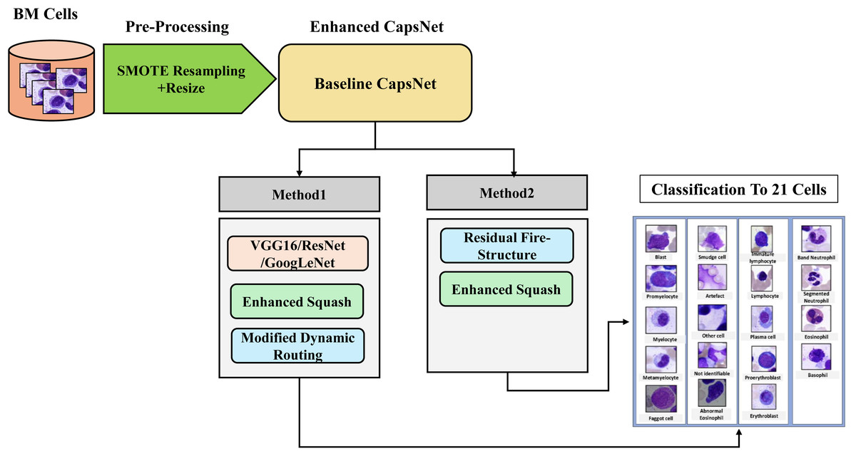
Figure 1: Methodology steps for classification.
Baseline CapsNet theory
The concept of CapsNet was initially proposed by Sabour, Frosst & Hinton (2017). These networks represent images in a whole vector format, which allows them to encode internal properties, including the pose of entities within an image. In contrast to CNNs, which rely on pooling for output routing, CapsNet aims to preserve information to achieve equivariance, particularly in handling viewpoint changes. This preservation is facilitated through dynamic routing, which replaces the pooling mechanism. Lower-level capsules representing specific features are hierarchically routed to parent capsules to capture part-whole relationships via linear transformations. This approach is based on the concept of inverse graphics, which suggests that the neural system deconstructs images into their inherent hierarchical properties. A capsule is a group of neurons that performs a diverse range of internal computations and subsequently encodes the results of these computations into an n-dimensional vector. The vector is the output of the capsule. The length of this output vector indicates the vector’s probability and direction, indicating specific properties about the entity. Using initial convolutional layers in capsule networks permits the reuse and replication of learned knowledge across different parts of the receptive field. An iterative Dynamic Routing algorithm is employed to determine the inputs to the capsules. The output of each capsule is then compared with the actual production of the higher-level capsules. In the case of a match between the outputs, the coupling coefficient between the two capsules is increased. Let represent a lower-level capsule and represent a higher-level capsule. The prediction vector is calculated as follows in Eq. (1):
(1) The trainable weighting matrix and the Output pose vector from the ( ) capsule to the ( ) Capsules are employed in this context. The coupling coefficients are calculated using a SoftMax function as follows in Eq. (2):
(2) The log probability of capsule i coupled with capsule j, denoted by bij, is initialized with zero values. The total input to capsule j is a weighted sum of the prediction vectors, calculated as follows in Eq. (3):
(3)
In capsule networks, the length of the output vector is employed to represent the probability for the capsule. Consequently, a non-linear activation function, the squashing function, is used. The squashing function is defined as follows in Eq. (4):
(4)
The dynamic routing algorithm can update the Values in each iteration. In this case, the objective is to optimize the Vj vector. In the dynamic routing algorithm, the The Vector is updated in every iteration according to Eq. (5):
(5)
Dataset
BM cell dataset (Matek et al., 2021), the dataset is available to the public, and there is no personal information in this, includes various hematological disease cell microscopic images consisting of more than 170,000 de-identified, expert-annotated cells from bone marrow smears of 961 patients stained using the May-Grünwald-Giemsa/Pappenheim stain. The institutional review board at the Munich Leukemia Laboratory (MLL) has given its permission to use this dataset. Sample microscopic images from the dataset are shown in Fig. 2.
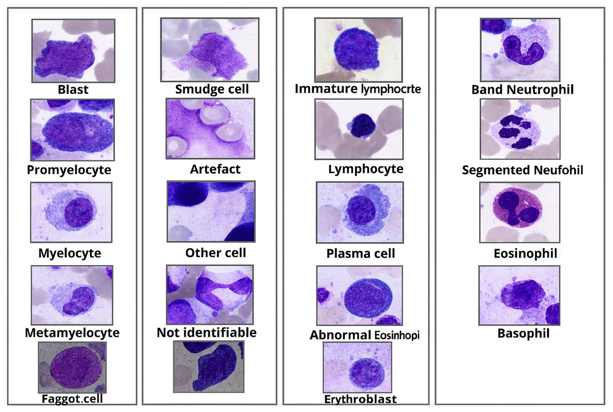
Figure 2: Morphological appearance of BM cell classes.
Pre-processing
As seen in Fig. 3, imbalances in the distribution of some BM cell dataset classes cannot reach the expected target. SMOTE (Chawla et al., 2011) Adaptive Synthetic (ADASYN) (He et al., 2008), SMOTEBoost (Chawla et al., 2003), and DataBoostIM (Guo & Viktor, 2004). Sampling approach techniques are used to avoid these imbalances.
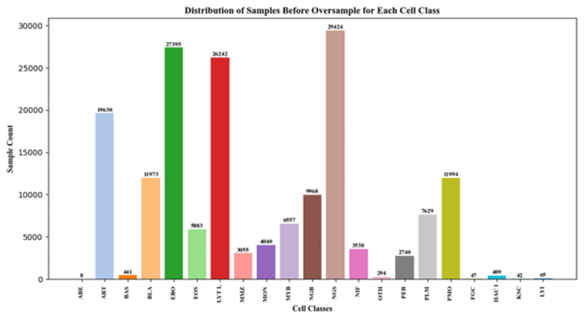
Figure 3: BM cell dataset features.
In this study, SMOTE, which is preferred over other sampling approximation techniques (Sci-Hub, 2019; Maldonado, López & Vairetti, 2019). It is used to create synthetic instances of the minority class by interpolating between class instances of an imbalanced dataset. Elreedy & Atiya (2019) using Eq. (6) (Reza & Ma, 2019; Juanjuan et al., 2007). In Eq. (6), it is the actual minority value. is the number of nearest neighbors of the actual value? is the nearest neighbor value does Euclidean distance obtain the difference? is the number value that allows the addition of different feature values. In this study, = 5 for each minority class.
(6)
Minority classes were rounded to 5,000 images, and classes with over 5,000 images were rounded up. This over-sampling technique improved overall classification performance and representation of the minority classes. Figure 4 shows the change in data points after the SMOTE process. In addition, all images are rescaled using bicubic interpolation (Wikipedia).
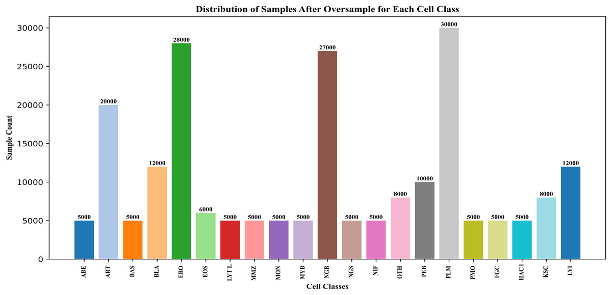
Figure 4: After oversampling the BM cell dataset features.
The primary reason that the classification performance is better is that SMOTE was used to balance the dataset before training. The models do not automatically deal with class imbalance. This technique is a non-adaptive interpolation algorithm and uses polynomial techniques to sharpen and enlarge digital images.
Baseline CapsNet model
The input images of the baseline CapsNet model were resized to 32 × 32 pixels to reduce the training time and then designed as shown in Fig. 5.
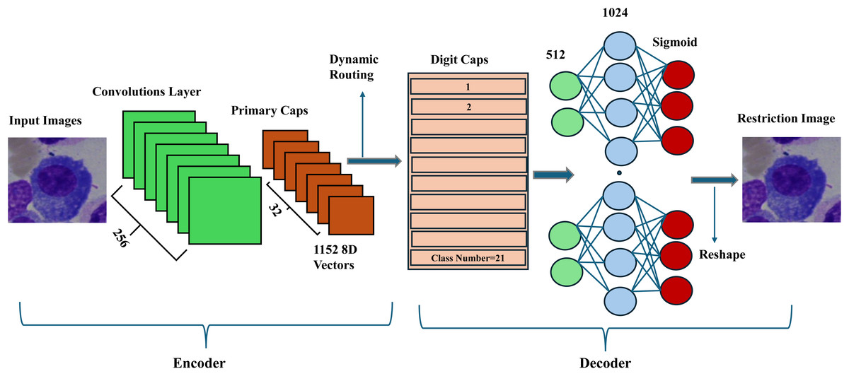
Figure 5: The general structure of the proposed CapsNet on the BM dataset.
The proposed model takes three arguments: the input image, the number of classes, and the number of routing iterations. After input images are preprocessed as in previous steps, they are fed to the convolutional layer to extract low-level features with filters of 256, kernel size 9, and strides of 1. Then, these features are grouped into primary capsules with filters of 8 × 32, kernel of 9 × 9, and stride of 1 to reduce the model size, each representing a part or aspect of an object. Each capsule in the convolutional layer corresponds to a capsule in the primary capsule layer. A routing-by-agreement approach boosts learning capability and captures the relationships between different parts of an object. Each capsule in a higher-level layer sends its output to capsules in the layer above based on the agreement (compatibility) between their outputs. The routing process consists of iteratively updating the connection weights between capsules based on the match between their outputs. Thus, dynamic routing makes the capsules in higher layers focus on the most relevant capsules in the layer below; the ReLU activation function, a non-linear function in deep neural networks, is used to reduce dimension. The output of the capsule network is obtained by measuring the length of the output vectors of the capsules in the top layer. This length indicates the probability that a given class or object is present in the input image. Standard squash is applied to squash the vectors of the primary capsules as a non-linear activation function. It aims to ensure that short vectors are reduced to a length close to zero and long vectors are reduced to a length close to 1. Then, adjusting the hyperparameter, the learning rate is initially determined to be 0.001, and the Adam (Kingma & Ba, 2014) optimization algorithm is used to change it dynamically. The model is run with a decay ratio of 0.9 and a routing of 3 for 100 epochs. The CapsNet model train accuracy is calculated at 96.99% on the BM dataset. Next, two powerful methods are proposed to enhance further the most important cores in the structure of the baseline CapsNet, such as squash, dynamic routing, and the feature extractor part.
Method 1: pretrained-CapsNet, custom squash, and modified dynamic
The proposed architecture, shown in Figs. 6, and 7, is pre-trained on ImageNet with the CapsNet architecture to extract features from the BM cell images after resizing the image to a 75 × 75 scale. These features are then fed into the primary convolution layer of the capsule layers with a filter size of 8 × 32, a stride of 2, and a kernel size of 1. The output of the Conv2D layer is reshaped to match the desired shape of the primary capsule layer, followed by the application of the enhanced equation of the squash function. The standard Squash function used in capsule networks compresses vector magnitudes to values between 0 and 1, while preserving direction as shown in Eq. (4) above. However, this approach is limited by its reliance on the L2 norm alone, which can result in vanishing gradients especially for vectors near their maximum length. It also struggles with minimal vectors, sensitivity to input scale and slow convergence. To address these limitations, we present an improved squash function that incorporates layer normalization and a scaling factor α.
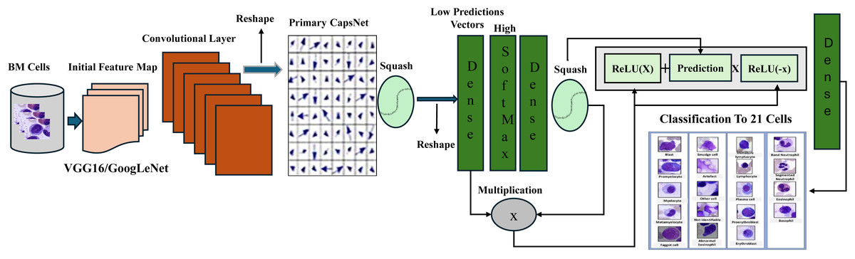
Figure 6: Structure of proposed pretrained-CapsNet on the BM dataset.
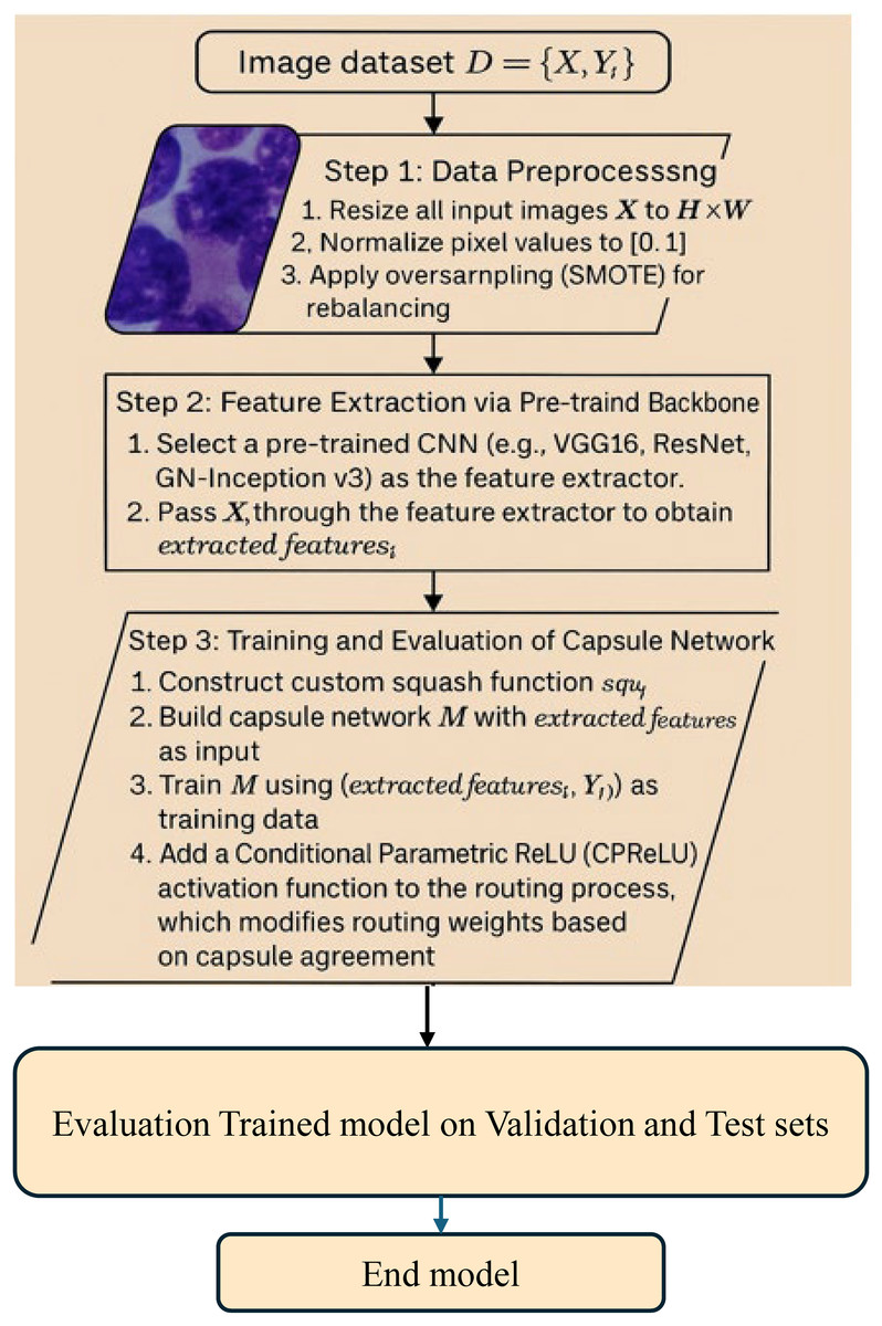
Figure 7: Algorithm 1—enhanced pre-trained capsule networks with conditional parametric ReLU (CPReLU).
This enhancement stabilizes learning by independently computing mean and variance for each capsule, centering, and scaling activations. The scaling factor is computed based on the squared L2 norm of the input vectors divided by 5. , using scaling , controls the intensity of squashing, and promotes scale invariance. In addition, layer normalization subtracts the meaning from the input vectors to center them around the zero mean, reducing variance and improving stability. Improved robustness is a further advantage of the enhanced function; it reduces sensitivity to parameter addition and internal covariate shift and enhances gradient flow and capsule network expressiveness. Using mean and variance instead of the standard function, layer normalization captures more information than simply the input vector’s squared norm. This better function speeds convergence, improves slopes, and lowers bias. It also allows more complex relationships in the data to be captured. The final equation combines scaling and normalization, providing a comprehensive approach to addressing the limitations of the standard squash function and improving the performance of CapsNet in tasks such as image classification and object detection. The enhanced squash is represented as:
(7)
(8)
(9) Here, is the capsule input vector, and are the mean and variance of the vector components, respectively, and is a small constant added for numerical stability. α = 0.5 was chosen through extensive experimentation as it produced the best results across multiple datasets. This value balances vector compression with sufficient dynamic range to improve convergence and model robustness. Including layer normalization ensures that each capsule’s output is centered and scaled individually, reducing internal covariate shift and promoting scale invariance. Compared to the original function, this enhancement improves training stability and speeds up convergence.
After squashing vectors, batch normalization (Santurkar et al., 2018) is applied with an impulse of 0.8 to maintain standardized output values. A dense layer called GN-Caps, consisting of 160 neurons, is initialized with He-normal and zero initializers for the kernel and bias, respectively, and processes the normalized output. Next, the routing algorithm is applied. Subsequent routing iterations include SoftMax activation and a dense layer of 160 neurons. The output vectors are then squashed. The element-wise multiplication of the squashed SoftMax output and the lower-level capsules (initially predicted vectors) is used to compute the routing weights between the lower and upper-level capsules and to further improve routing performance. The result is then passed through a CPReLU. (This extends to PReLU (Krstić et al., 2021)). We introduce the CPReLU activation function to the dynamic routing process. Unlike standard ReLU or PReLU, CPReLU uses routing predictions (e.g., SoftMax outputs) as a conditional parameter for adapting negative activations.
This allows the model to adjust how it handles negative activations based on the incoming data.
(10)
CPReLU replaces the static slope parameter α with a dynamic ( ), enabling instance-specific adaptation. The CPReLU function uses the following enhanced equations:
(11)
(12) When input (x) is not negative, it returns x, unchanged. If x is negative, it sums predictions scaled by the maximum of 0 and the negative value of input (x).
While PReLU provides a global slope adjustment for negative inputs across the network, conditional PReLU provides a more localized and adaptive adjustment on a per-neuron basis, allowing for greater flexibility and potentially better model fit. We suggest adding a CPReLU activation function to the routing process, which is different from the traditional dynamic routing mechanism in capsule networks, where the capsule outputs are updated without activation-aware modification. In our method, the routing weights are changed not just by capsule agreement but also by softmax-based predictions, which act as conditional coefficients in the CPReLU function. This architecture lets the network change the size of negative activations depending on how sure it is about routing assignments. This makes capsule updates more non-linear and sensitive to input. The CPReLU function lets you change the way it works according to where the data is coming from. This helps reduce dead neurones, speeds up routing convergence, and better captures complex information connections, especially in datasets that are noisy or imbalanced.
The output of the final routing iteration passes through a 32-neuron dense layer before being predicted using a dense layer with the number of neurons equal to the 21 classes of the dataset, with Softmax activation to generate class probabilities. The GN-CapsNet model combines Google Inception V3 (Cloud, 2024). With CapsNet to take advantage of Inception V3’s ability to capture features at multiple scales and the efficiency of CapsNet in handling complex relationships within data. In the VGG-CapsNet model, which combines VGG16 with CapsNet, the VGG-CapsNet model is proposed to exploit the feature extraction capabilities of VGG16, which excels at learning hierarchical features from images and RES-CapsNet is combined ResNet152V2 (Researchgate). With CapsNet. The models were trained using categorical cross-entropy loss and the Adam optimizer, with hyperparameters such as learning decay (0.9), learning rate (0.001), and normalization momentum (0.8) tuned for optimal performance after establishing Pretrained-CapsNet architecture.
Method 2: Fire-CapsNet
The presented architecture is shown in Figs. 8 and 9. The implementation of Fire-CapsNet in the method follows a hierarchical structure with three main components: Base Filter Substructure (BFS): This is the first stage that performs basic feature extraction from the input image.
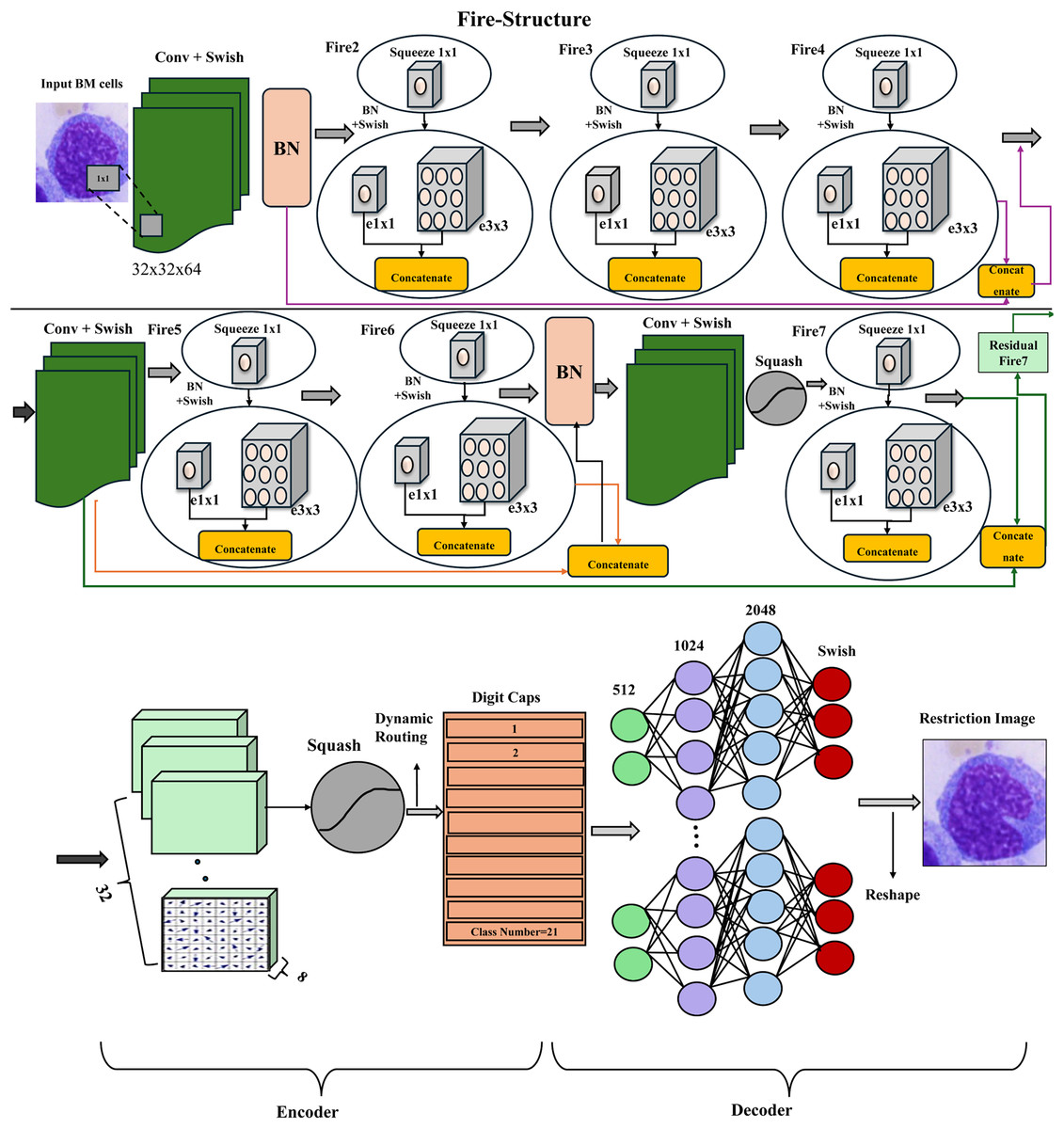
Figure 8: Structure of proposed Fire-CapsNet on the BM dataset.
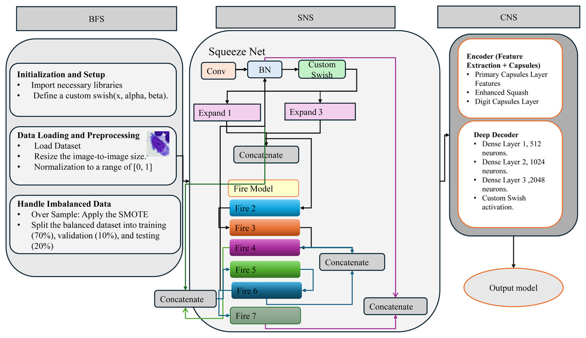
Figure 9: Algorithm workflow of the proposed enhanced Fire-CapsNet model.
A convolutional layer with a small kernel size (1 × 1) with a custom Swish activation function using multiple parameters, such as ( They are used to extract low-level features such as edges and corners. (scaling factor): This adjusts the total range of the function’s output. A value of α greater than 1 would amplify positive outputs, while a value between 0 and 1 would compress them. β (Sigmoid Steepness): This controls how sharply the function transitions from negative to positive values. Thus, a higher β produces a steeper transition.
To address the limitations of standard activation functions, such as ReLU, or standard swish which can result in dead neurons and non-smooth gradients, we have developed a customized Swish activation function for Fire-CapsNet architecture.
The custom or enhanced swish is computed as:
(13) where σ is the sigmoid function and α and β are trainable or fixed scaling parameters. This modified Swish activation function: preserves gradient flow across layers due to its smooth, non-monotonic shape. It enhances learning stability and generalization, especially in deep networks. It is also more robust than ReLU when applied in Fire modules and capsule layers.
Further, Batch normalization is applied to improve the stability of the training. Second components of structure squeeze net (SNS): This section incorporates Fire modules, a technique for efficient feature extraction. The fire module is a building block of the Squeeze Net (Trending Papers) Architecture. However, the standard fire method has been modified in this method. It starts with a 1 × 1 convolutional layer (squeeze) to reduce the number of input channels (squeeze the input). Batch normalization is applied to normalize the activation of the layer. The Swish activation function (implemented as a custom swish) introduces non-linearity. It then separates into two branches. Expand1 A 1 × 1 convolutional layer to increase the number of channels. Expand3 branch: A 3 × 3 convolutional layer to capture spatial information. The outputs of the Expand1 and Expand3 branches are concatenated along the channel axis. After seven fire modules are used, a residual connection is used to preserve information flow and facilitate the training of deeper networks. For example, after fire4, there is a residual connection from the input (BN1) to the output (fire4), similarly, after the second convolution, a residual connection to fire6. In standard fire models, max pooling is often used for down sampling, which can result in a loss of information. This implementation replaces max pooling with a convolutional layer with a stride greater than 1. While ResNet employs identity or convolution-based skip connections between standard convolution layers, Fire-CapsNet integrates residual connections across modular Fire blocks, enabling lightweight yet effective feature reuse. Additionally, Fire-CapsNet extends residual connections into the capsule routing structure, a design not found in traditional residual networks like ResNet. This not only improves gradient flow but also enhances capsule-based representation learning. This stride reduces the spatial dimensions of the feature maps while preserving more information than max pooling as shown in Table 1.
| Aspect | Modified fire model | Standard fire module |
|---|---|---|
| Expand layer 1 | 1 × 1 Convolutional layer + Batch normalization + Custom swish | 1 × 1 Convolutional layer + ReLU |
| Expand layer 2 | 3 × 3 Convolutional layer + Batch normalization + Custom swish | 1 × 1 or 3 × 3 Convolutional layer + ReLU |
| Activation function | Custom swish | ReLU |
| Down sampling | Conv2D with strides = (2, 2) | Max-pooling layers |
| Residual connection | Yes | No |
The third component in this method is CapsNet Substructure (CNS): This core component introduces capsule layers. The primary capsule layer transforms the extracted features into capsules with a filter size of 8 × 32, a stride of 2, and a kernel size of 1. The output of the Conv2D layer is reshaped to match the desired shape of the primary capsule layer. An enhanced squash activation function is then employed to limit the capsule activations between 0 and 1. The digit capsule layer performs routing iterations to learn the relationships between the capsules and predict the image’s class probability. Finally, a deep decoder part is added to the CapsNet model, including a dropout layer with a dropout rate of 0.3 for regularization. The decoder consists of dense layers of 512, 1,024, 2,048, and output neurons, custom swish activation, and batch normalization. It is designed to reconstruct the input images from the capsule outputs, ensuring that the model encodes meaningful information and reduces overfitting. The models were trained using loss margin and the Adam optimizer, with hyperparameters such as learning decay (0.9), learning rate (0.001), and normalization momentum (0.8) tuned for optimal performance after establishing the Fire-CapsNet architecture. The proposed Fire-CapsNet is better than standard CapsNet because it adds lightweight Fire modules from SqueezeNet to make multi-scale feature extraction more efficient. Residual connections are established between Fire blocks and the first layers to improve the flow of gradients and the reuse of features. A custom Swish activation algorithm makes gradients smoother and increases non-linearity. These improvements lead to improved representation, faster convergence, and higher accuracy on substantial, unbalanced datasets.
Experimental results and discussion
Using 128 GB RAM, 8 GB VRAM and NVIDIA RTX 3070 GPU, we trained and evaluated our models. This offered sufficient computing capability. The models’ development handled large datasets and complex characteristics. Furthermore, datasets can be used with them. These models have wide applications in many medical domains because they can handle imbalanced classes in medical datasets.
Evaluation process of models
It analyzed a large collection of BM cell images using the pre-trained CapsNet model. This provides an opportunity to show the effects of the modification methods and assess how well the model classified BM cells. Important measures of classification accuracy covering several facets were used to evaluate the model’s performance: precision, specificity, recall, and F1-score. These measurements were computed with formulas, as will be explained below:
(14)
(15)
(16)
(17)
Results
This part evaluates, with publicly available datasets, the performance of our enhanced models for BM cell classification. The Oversampling techniques SMOTE approach addresses the class imbalance in the BM cell dataset. Our models’ accuracy increased when SMOTE was included during training with SMOTE. 171,374 images were included in the original dataset. Then, SMOTE was used to create 216,000 BM images. The dataset was split into 70% for training, 10% for validation, and 20% for testing, as shown in Table 2. Further, we evaluated three more datasets: MNIST, Fashion MNIST, and CIFAR-10. These datasets present challenges and help us understand how our model performs in different applications. The MNIST dataset contains images of handwritten digits, which are used to test image classification. The Fashion MNIST dataset includes images of clothes and accessories. The Fashion MNIST dataset is more complex than the MNIST dataset. Our models recognized more complex characteristics and small differences among fashion items. The CIFAR-10 dataset is a 10-classification problem with a broader spectrum of object classes. The increased complexity and variability of CIFAR-10 provides a challenging environment. Table 3 shows the details of these three datasets.
| Total BM cells | After applying SMOTE | Training data (70%) | Validation (10%) | Test data (20%) |
|---|---|---|---|---|
| 171,374 | 216,000 | 151,200 | 21,600 | 43,200 |
| Dataset | Image size | Channels | Classes | Train set | Test set |
|---|---|---|---|---|---|
| MNIST | (28, 28) | 1 | 10 | 60,000 | 10,000 |
| Fashion-MNIST | (28, 28) | 1 | 10 | 60,000 | 10,000 |
| Cifar10 | (32, 32) | 3 | 10 | 50,000 | 10,000 |
Method 1 results
The performance metrics of the pre-trained CapsNet model show exceptional results across different classes of BM cells. The precision, recall, specificity, and F1-score metrics show consistently high values, as shown in Tables 4, 5, 6, and 7. indicating the ability of the models to classify different cell types with high accuracy. Baseline CapsNet performance is less effective than other models in pre-trained models; Classes such as ABE, ART, BAS, BLA, and FGC achieve perfect scores across all metrics, demonstrating the model’s ability to identify these cell types accurately.
| Class name | Precision (%) | Recall (%) | Specificity (%) | F1-score (%) |
|---|---|---|---|---|
| ABE | 100 | 100 | 100 | 100 |
| ART | 100 | 100 | 100 | 100 |
| BAS | 100 | 100 | 100 | 100 |
| BLA | 99.92 | 100 | 100 | 99.96 |
| EBO | 99.89 | 99.96 | 99.98 | 99.93 |
| EOS | 100 | 99.5 | 100 | 99.75 |
| FGC | 100 | 100 | 100 | 100 |
| HAC | 100 | 100 | 100 | 100 |
| KSC | 100 | 100 | 100 | 100 |
| LYI | 100 | 100 | 100 | 100 |
| LYT | 99.17 | 99.59 | 99.88 | 99.38 |
| MMZ | 95.03 | 89.8 | 99.89 | 92.34 |
| MON | 89.01 | 89.1 | 99.74 | 89.06 |
| MYB | 92.57 | 93.37 | 99.71 | 92.97 |
| NGB | 91.74 | 85 | 99.63 | 88.24 |
| NGS | 94.19 | 97.47 | 99.03 | 95.8 |
| NIF | 91.86 | 86.9 | 99.82 | 89.31 |
| OTH | 97.35 | 99.1 | 99.94 | 98.22 |
| PEB | 95.35 | 92.3 | 99.89 | 93.8 |
| PLM | 93.28 | 86.75 | 99.76 | 89.9 |
| PMO | 91.83 | 97 | 99.49 | 94.35 |
| Class name | Precision (%) | Recall (%) | Specificity (%) | F1-score (%) |
|---|---|---|---|---|
| ABE | 100 | 100 | 100 | 100 |
| ART | 100 | 100 | 100 | 100 |
| BAS | 100 | 100 | 100 | 100 |
| BLA | 99.96 | 100 | 100 | 99.98 |
| EBO | 99.79 | 99.96 | 99.97 | 99.88 |
| EOS | 99.92 | 99 | 100 | 99.46 |
| FGC | 100 | 100 | 100 | 100 |
| HAC | 100 | 100 | 100 | 100 |
| KSC | 100 | 100 | 100 | 100 |
| LYI | 100 | 100 | 100 | 100 |
| LYT | 99.78 | 99.76 | 99.97 | 99.77 |
| MMZ | 97.59 | 97.3 | 99.94 | 97.45 |
| MON | 96.4 | 96.5 | 99.91 | 97.45 |
| MYB | 97.51 | 97.81 | 99.9 | 98.66 |
| NGB | 96.67 | 95.89 | 99.79 | 96.39 |
| NGS | 98.3 | 98.57 | 99.73 | 98.44 |
| NIF | 97.89 | 97.3 | 99.95 | 97.59 |
| OTH | 99.6 | 99.9 | 99.99 | 99.75 |
| PEB | 97.5 | 97.6 | 99.94 | 98.55 |
| PLM | 98.2 | 96.69 | 99.93 | 96.93 |
| PMO | 97.58 | 99.08 | 99.86 | 98.33 |
| Class name | Precision (%) | Recall (%) | Specificity (%) | F1-score (%) |
|---|---|---|---|---|
| ABE | 100 | 100 | 100 | 100 |
| ART | 100 | 100 | 100 | 100 |
| BAS | 100 | 100 | 100 | 100 |
| BLA | 100 | 100 | 100 | 100 |
| EBO | 99.98 | 100 | 100 | 99.99 |
| EOS | 100 | 99.92 | 100 | 99.96 |
| FGC | 100 | 100 | 100 | 100 |
| HAC | 100 | 100 | 100 | 100 |
| KSC | 100 | 100 | 100 | 100 |
| LYI | 99.9 | 100 | 100 | 99.95 |
| LYT | 99.94 | 99.89 | 99.99 | 98.92 |
| MMZ | 97.92 | 98.8 | 99.95 | 99.36 |
| MON | 96.74 | 97.8 | 99.92 | 97.27 |
| MYB | 98.74 | 98.19 | 99.95 | 98.46 |
| NGB | 96.08 | 96.85 | 99.81 | 97.46 |
| NGS | 98.77 | 98.63 | 99.8 | 98.7 |
| NIF | 98.98 | 98.2 | 99.98 | 98.08 |
| OTH | 99.4 | 100 | 99.99 | 99.7 |
| PEB | 98.6 | 98.3 | 98.97 | 98.45 |
| PLM | 97.57 | 97.88 | 99.91 | 97.72 |
| PMO | 98.96 | 98.67 | 99.94 | 98.81 |
Note:
The precision, recall, specificity, and F1-score metrics show consistently high values, as shown in Table 6.
| Class name | Precision (%) | Recall (%) | Specificity (%) | F1-score (%) |
|---|---|---|---|---|
| ABE | 100 | 100 | 100 | 100 |
| ART | 100 | 100 | 100 | 100 |
| BAS | 100 | 100 | 100 | 100 |
| BLA | 100 | 100 | 100 | 100 |
| EBO | 99.96 | 99.98 | 99.99 | 99.97 |
| EOS | 99.92 | 99.83 | 100 | 99.87 |
| FGC | 100 | 100 | 100 | 100 |
| HAC | 100 | 100 | 100 | 100 |
| KSC | 100 | 100 | 100 | 100 |
| LYI | 100 | 100 | 100 | 100 |
| LYT | 99.91 | 99.96 | 99.99 | 98.94 |
| MMZ | 98.8 | 99 | 99.97 | 98.9 |
| MON | 98.59 | 97.91 | 99.96 | 98.04 |
| MYB | 98.39 | 99.25 | 99.94 | 98.82 |
| NGB | 96.77 | 98.45 | 99.84 | 98.11 |
| NGS | 99.08 | 98.85 | 99.85 | 98.97 |
| NIF | 99.26 | 97.8 | 99.98 | 98.54 |
| OTH | 99.6 | 100 | 99.99 | 99.8 |
| PEB | 98.32 | 99.5 | 99.96 | 99.91 |
| PLM | 98.87 | 98.5 | 99.96 | 98.69 |
| PMO | 99.67 | 99.38 | 99.98 | 99.52 |
The results presented in Table 8 provide a comparative analysis between the baseline CapsNet model and its enhanced versions, VGG-CapsNet and GN-CapsNet, on the BM datasets. The baseline CapsNet achieves an accuracy of 96.99%, requires 100 epochs, and takes approximately 3 h and 22 min to train. In contrast, the improved models show significant improvements in several aspects. All pretrained-CapsNet outperform the baseline model, achieving accuracies of 99.31%, 99.38% and 99.89%, VGG-CapsNet, RES-CapsNet, and GN-CapsNet, respectively. This considerable increase in accuracy highlights the effectiveness of the enhancements incorporated into these models. In addition, all improved models require only 50 epochs to reach convergence, halving the number of epochs needed for the baseline CapsNet. This faster convergence indicates the improved training efficiency introduced by the modifications. In addition, training time is significantly reduced, with VGG-CapsNet completing training in 1 h 20 min, RES-CapsNet in 4 h, and GN-CapsNet completing training in 1 h 33 min, as shown in Table 8. These reductions in training time and improved accuracy highlight the superior performance of the models, as shown in Fig. 10.
| Method | Accuracy (%) | Number of epochs | Time running (h) |
|---|---|---|---|
| Baseline CapsNet | 96.99 | 100 | 3:22:00 |
| VGG-CapsNet | 99.31 | 50 | 1:20:00 |
| RES-CapsNet | 99.38 | 50 | 4:01:00 |
| GN-CapsNet | 99.89 | 50 | 1:33:00 |
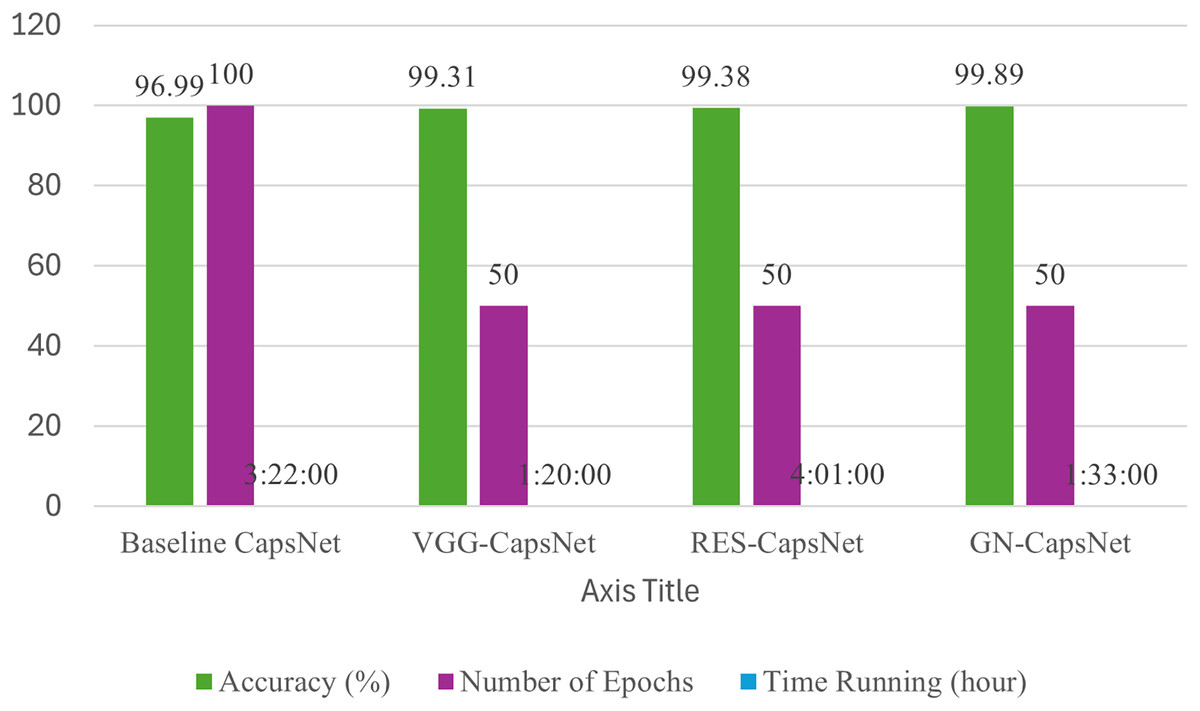
Figure 10: Accuracy comparison of baseline CapsNet and enhanced CapsNet on BM datasets.
The results in Table 9 below demonstrate the performance of different CapsNet architectures. In the CIFAR-10 dataset, the baseline CapsNet achieves an accuracy of 67.81%. VGG-CapsNet achieves an accuracy of 83.58%, showing a significant improvement. Res-CapsNet slightly outperforms with an accuracy of 84.02%, demonstrating the benefits of residual connections in improving feature learning. The highest performance is achieved by GN-CapsNet with an accuracy of 86.54%, highlighting the effectiveness of integrating global and residual learning mechanisms. For the Fashion MNIST dataset, which presents a more challenging, the baseline CapsNet achieves an accuracy of 92.49%, which is quite robust for this dataset. However, the advanced architectures again show significant improvements: VGG-CapsNet reaches 95.22%, Res-CapsNet reaches 95.46%, and GN-CapsNet reaches 95.95%. Finally, the MNIST dataset, known for its simplicity and low complexity, provides a benchmark where even traditional models achieve high accuracy. The baseline CapsNet performs very well, with an accuracy of 99.23%. However, the VGG-CapsNet, Res-CapsNet, and GN-CapsNet architectures perform even better, achieving 99.87%, 99.91%, and 99.93% accuracy, respectively as shown in Fig. 11.
| Dataset | Baseline capsnet | Vgg-Capsnet | Res-Capsnet | GN-capsnet |
|---|---|---|---|---|
| MNIST (Sabour, Frosst & Hinton, 2017) | 99.23% | 99.87% | 99.91 | 99.93% |
| Fashion MNIST (Afriyie, Weyori & Opoku, 2022c) | 92.49% | 95.22% | 95.46 | 95.95% |
| Cifar10 (El Alaoui-Elfels & Gadi, 2022) | 67.81% | 83.58% | 84.02 | 86.54% |
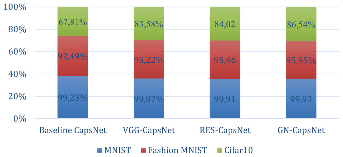
Figure 11: Accuracy comparison of baseline CapsNet and enhanced CapsNet on different datasets.
Figure 11 illustrates the accuracy curve for the enhanced CapsNet models on the training data across 50 epochs for GN-CapsNet and VGG-CapsNet and 100 epochs for baseline CapsNet. This curve demonstrates how the model’s classification accuracy evolves as training progresses. Figure 12 provides insights into the model’s dynamics and ability to improve accuracy over successive epochs.
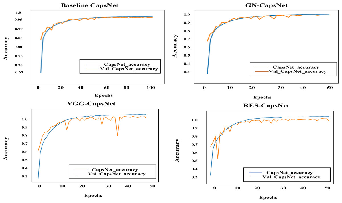
Figure 12: Accuracy curve comparison: baseline CapsNet, VGG-CapsNet, RES-CapsNet, and GN-CapsNet, on the BM dataset.
Method 2 results
The high precision, recall, specificity, and F1-scores of the Fire-CapsNet model are illustrated in Table 10 by the performance metrics for different classes. The model’s excellent results on all measures showed that classes such as ABE, ART, BAS, BLA, FGC, and HAC were particularly well-classified.
| Class name | Precision (%) | Recall (%) | Specificity (%) | F1-score (%) |
|---|---|---|---|---|
| ABE | 100 | 100 | 100 | 100 |
| ART | 100 | 100 | 100 | 100 |
| BAS | 100 | 100 | 100 | 100 |
| BLA | 100 | 100 | 100 | 100 |
| EBO | 99.96 | 99.98 | 99.99 | 99.98 |
| EOS | 99.92 | 99.83 | 100 | 99.87 |
| FGC | 100 | 100 | 100 | 100 |
| HAC | 100 | 100 | 100 | 100 |
| KSC | 100 | 100 | 100 | 99.99 |
| LYI | 100 | 100 | 100 | 100 |
| LYT | 99.91 | 99.96 | 99.99 | 99.94 |
| MMZ | 98.8 | 99 | 99.97 | 99.9 |
| MON | 98.59 | 97.91 | 99.96 | 98.04 |
| MYB | 98.39 | 99.25 | 99.94 | 99.82 |
| NGB | 97.77 | 98.45 | 99.84 | 99.11 |
| NGS | 99.08 | 98.85 | 99.85 | 98.97 |
| NIF | 99.26 | 97.8 | 99.98 | 99.54 |
| OTH | 99.6 | 100 | 99.99 | 99.8 |
| PEB | 98.32 | 99.5 | 99.96 | 99.91 |
| PLM | 98.87 | 98.5 | 99.96 | 99.69 |
| PMO | 99.67 | 99.38 | 99.98 | 99.52 |
MNIST dataset in Table 11 achieves the highest accuracy, 99.95%, indicating that the model has learned the patterns in the dataset very well. Fashion-MNIST follows close behind with an accuracy of 95.98%, indicating that the model can generalize similar image recognition tasks well with different categories. Cifar10 has a slightly lower accuracy (90.02%) than the previous two datasets. BM achieves 99.92% accuracy. These results are after 20 epochs for all datasets. It is important to consider that the better classification performance on the BM dataset isn’t just because of proposed model architecture: it is also because SMOTE was used during preprocessing. It is important to note that the optimal number of epochs can vary depending on the complexity of the model, as shown in Figs. 13 and 14.
| Dataset | Accuracy | Number of epochs |
|---|---|---|
| MNIST | 99.95 | 20 |
| Fashion MNIST | 95.98 | 20 |
| Cifar10 | 90.02 | 20 |
| BM | 99.92 | 20 |
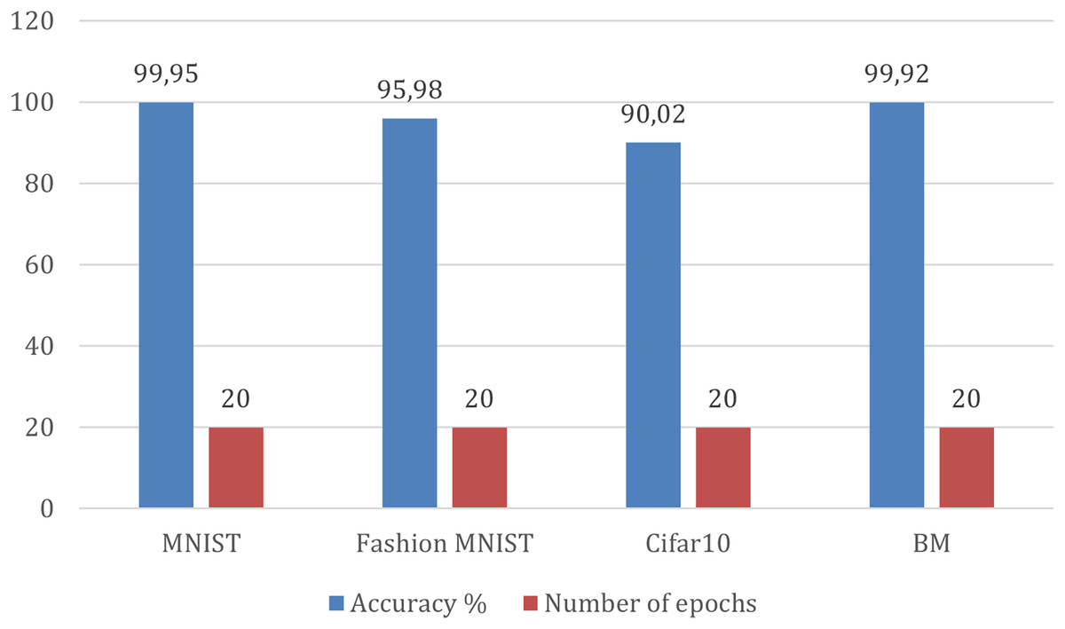
Figure 13: Accuracy comparison of Fire-CapsNet on different datasets.
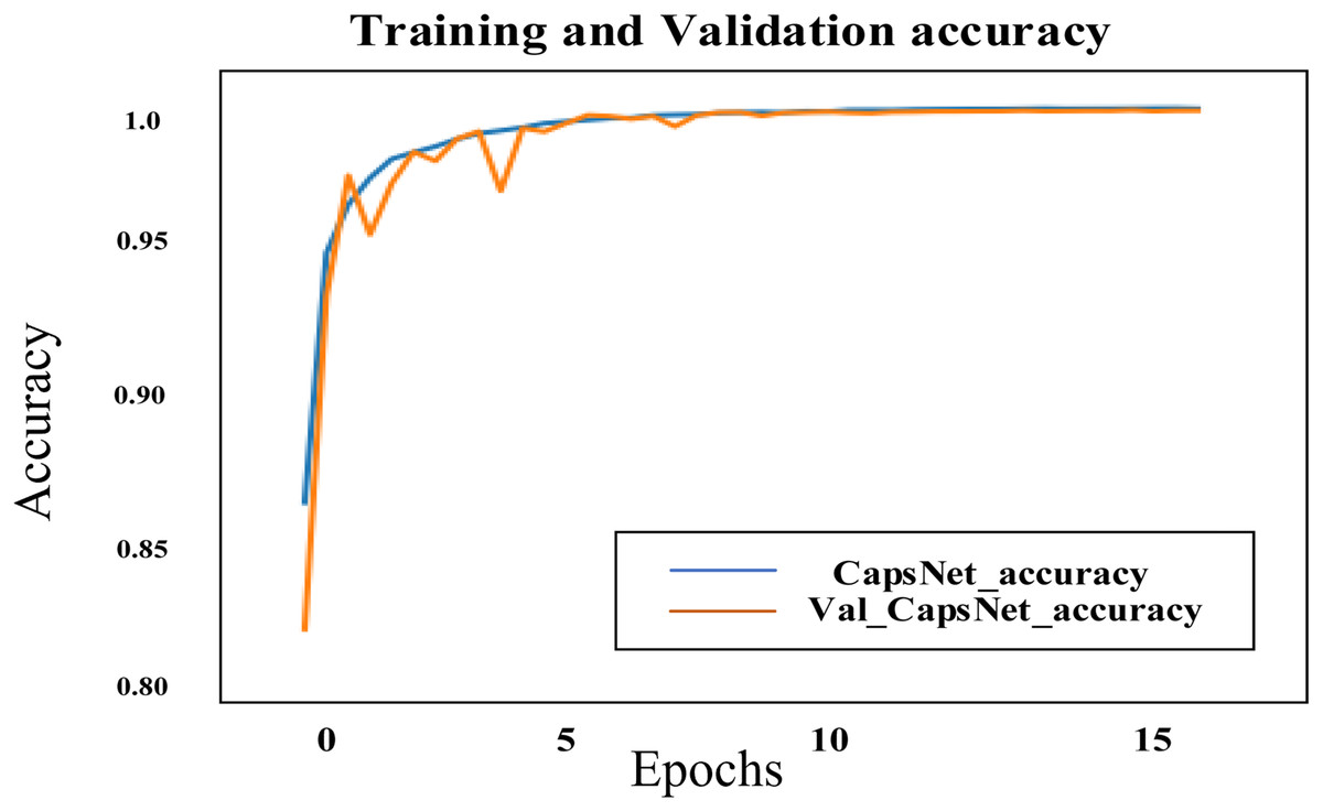
Figure 14: Accuracy curve of Fire-CapsNet on the BM dataset.
Comparison of our models with other proposed models and state-of-the-art methods
Table 12 below shows the performance of several proposed enhanced CapsNet models on four different datasets, including MNIST, Fashion-MNIST, CIFAR-10, and a dataset labelled “BM”. Each model is trained on a different number of epochs, ranging from 20 to 100, and the models trained with Method and Method2 consistently outperform the Baseline CapsNet, with Method2 achieving the highest accuracy of 99.91% at 20 epochs on BM, demonstrating its effectiveness in improving model performance. Fashion MNIST dataset and MNIST dataset, all proposed models show higher accuracy compared to the baseline CapsNet. The Fire-CapsNet model trained with Method 2 achieves the highest accuracy of 90.02% with the Cifar10 dataset, demonstrating its effectiveness in handling more complex image datasets.
| Dataset | Method1 Epochs = 50 | Method2 Epochs = 20 | |||
|---|---|---|---|---|---|
| Baseline CapsNet Epochs = 100 | VGG-Caps | RES-CapsNet | GN-CapsNet | Fire-CapsNet | |
| MNIST | 99.23 | 99.87 | 99.91 | 99.93 | 99.95 |
| Fashion-MNIST | 92.49 | 95.22 | 95.46 | 95.95 | 95.98 |
| Cifar10 | 67.81 | 83.58 | 84.02 | 86.54 | 90.02 |
| BM | 96.66 | 99.31 | 99.38 | 99.89 | 99.92 |
Table 13 comprehensively compares different CapsNet architectures across multiple datasets, including MNIST, Fashion MNIST, CIFAR-10, and BM. The proposed model, particularly method 3 (Fire-CapsNet), achieves the highest accuracy of 99.95%, outperforming other CapsNet architectures and the different proposed models and CapsNet baselines.
| Methods | MNIST (%) | Fashion MNIST (%) | Cifar10 (%) | BM (%) |
|---|---|---|---|---|
| ShallowNet (Mensah, Weyori & Ayidzoe, 2021) | – | 92.70 | 75.75 | – |
| CapsNet (Sabour, Frosst & Hinton, 2017) | 90.72 | 62.91 | – | |
| Enhanced-CapsNet (Sabour, Frosst & Hinton, 2017) | 99.65 | – | 82.31 | – |
| 64 Capsule Layers (Xi, Bing & Jin, 2024) | 68.93 | – | 64.67 | – |
| Feature Amplification CapsNet (Ayidzoe et al., 2021b) | 93.76 | 84.56 | – | |
| Multi-lane (Chang & Liu, 2020) | 99.73 | 92.63 | 76.79 | – |
| MS-CapsNet (Xiang et al., 2018) | 92.70 | 75.70 | – | |
| ResCapsNet (Goswami, 2019) | – | 78.54 | – | |
| CFC-CapsNet (Shiri & Baniasadi, 2021) | – | 92.86 | 73.15 | – |
| Fast Inference (Zhao et al., 2019) | 99.43 | 91.52 | 70.33 | – |
| Inverted dot product (Tsai et al., 2020) | – | 82.55 | – | |
| Max–min (Zhao et al., 2019) | 99.55 | 92.07 | 75.92 | – |
| Quaternion CapsNet (Özcan, Kinli & Kiraç, 2021) | – | 90.26 | 82.21 | – |
| Gabor capsNet with prep blocks (Ayidzoe et al., 2021a) | – | 94.78 | 85.24 | – |
| MLSCN (Chang & Liu, 2020) | 99.73 | – | 76.79 | – |
| DeeperCaps (Xiong et al., 2019) | 99.84 | – | 81.29 | – |
| MLCN (do Rosario, Breternitz & Borin, 2021) | – | 92.63 | 75.18 | – |
| Cv-CapsNet++ (Cheng et al., 2024) | – | 94.40 | 86.70 | – |
| Quick-CapsNet (QCN) (Shiri, Sharifi & Baniasadi, 2020) | 99.28 | 88.84 | 67.18 | – |
| R-CapsNet (Luo, Duan & Wang, 2019) | – | 93.89 | 81.57 | – |
| SqueezeCapsNet (Adu et al., 2024) | 99.87 | 93.49 | 82.45 | – |
| Afriyie, Weyori & Opoku (2022b) | – | 92.80 | 75.42 | – |
| MCNet (Xu et al., 2024) | 99.63 | 93.17 | 79.27 | – |
| Afriyie, Weyori & Opoku (2022a) | – | 94.93 | 84.57 | – |
| Proposed models | ||||
| Method1: | ||||
| VGG-CapsNet | 99.87 | 95.22 | 83.58 | 99.31 |
| RES-CapsNet | 99.91 | 95.46 | 84.02 | 99.38 |
| GN-CapsNet | 99.93 | 95.95 | 86.54 | 99.89 |
| Method 2: | ||||
| Fire-CapsNet | 99.95 | 95.98 | 90.02 | 99.92 |
As shown in Table 14, the studies on this BM dataset are limited because it is new and has huge, unbalanced data, but these issues have been solved in our proposed models. Previous methods, such as ResNeXt-50 and SWAV, achieved F1-scores (62–73%) higher than other methods, according to a performance comparison on the BM dataset. Our proposed models increased accuracy significantly, including Enhanced CapsNet architectures; Fire-CapsNet reached 99.92%.
| Reference | Year | Method | Performance metric | Result rate |
|---|---|---|---|---|
| Ananthakrishnan et al. (2022) | 2022 | CNN + SVM, CNN + XGB | Accuracy | 32%, 28% |
| Siamese neural | Accuracy | 91% | ||
| Fazeli et al. (2022) | 2022 | Supervised method (ResNeXt-50) | (Avg) F1-score | 62% |
| Precision | 68.24% | |||
| Recall | 72.92% | |||
| Self-supervised method (SW AV) | (Avg) F1-score | 73% | ||
| Precision | 78% | |||
| Recall | 70% | |||
| Supervised contrastive | (Avg) F1-score | 69% | ||
| Precision | 75% | |||
| Recall | 66% | |||
| Proposed model Method1 | 2024 | VGG-CapsNet, | Accuracy | 99.31% |
| RES-CapsNet | 99.38% | |||
| GN-CapsNet | 99.89% (50 epochs) | |||
| Proposed model Method2 | Fire-CapsNet | Accuracy | 99.92% (20 epochs) |
Conclusions
This study addresses the limitations inherent in the baseline CapsNet model to improve its performance. Each proposed model addresses these challenges by offering innovative solutions to specific weaknesses. Furthermore, comparing several CapsNet-based models on four datasets shows that Fire-CapsNet demonstrated superior performance across the evaluated datasets, based on the reported metrics and shortest training time in our experiments. Despite more recent models like VGG-Caps, RES-CapsNet, and GN-CapsNet much outperforming the baseline CapsNet, which was trained for 100 epochs, it still produces acceptable outcomes. Remarkably, the models preserve competitive accuracy even at fewer training epochs (Method 1 at 50 and Method at 20), underscoring the effectiveness of these sophisticated designs. This analysis highlights how crucial practical training is to achieve high model performance, as is architectural innovation. Using fire modules and innovative architectural designs, Fire-CapsNet not only outperforms other proposed models in terms of accuracy but also demonstrates significant improvements in training time. Remarkably perfect results are typically achieved by Fire-CapsNet, which excels especially at managing complicated data, huge datasets, and even small datasets, unbalanced complex datasets. Future work will aim to implement Fire-CapsNet for real-time applications.