Downscaling MODIS land surface temperature to 90 m using random forest regression to assess transferability
- Published
- Accepted
- Received
- Academic Editor
- Davide Chicco
- Subject Areas
- Artificial Intelligence, Data Mining and Machine Learning, Data Science, Spatial and Geographic Information Systems
- Keywords
- Spatiotemporal trade-off, Satellite sensors, Downscaling, Random forest regression, Land surface temperature, Spatial resolution, XGBoost, CatBoost
- Copyright
- © 2025 Das et al.
- Licence
- This is an open access article distributed under the terms of the Creative Commons Attribution License, which permits unrestricted use, distribution, reproduction and adaptation in any medium and for any purpose provided that it is properly attributed. For attribution, the original author(s), title, publication source (PeerJ Computer Science) and either DOI or URL of the article must be cited.
- Cite this article
- 2025. Downscaling MODIS land surface temperature to 90 m using random forest regression to assess transferability. PeerJ Computer Science 11:e3246 https://doi.org/10.7717/peerj-cs.3246
Abstract
The observable spatiotemporal trade-offs among different satellite sensors necessitate the downscaling of optical and thermal data to identify Earth’s surface features and analyze temperature variations at finer scales. This study employs a random forest (RF) regression model to downscale Moderate Resolution Imaging Spectroradiometer (MODIS) land surface temperature (LST) data from a 1-km spatial resolution to 90 m. The model is trained on a primary region and applied to a spatially distinct secondary region to evaluate its transferability. Six acquisition dates, each representing a different month, were selected for downscaling. For contextual performance assessment, eXtreme Gradient Boosting (XGBoost) and Categorical Boosting (CatBoost) models were also trained and evaluated using the same setup. In the primary region, the RF model showed minimal root mean square error (RMSE) deviation across all acquisition dates, underscoring the importance of incorporating multiple variables. Comparable performance was observed with XGBoost and CatBoost in the primary region. In the secondary region, RF demonstrated strong generalizability, with the lowest RMSEs recorded in November (0.85) and February (0.96), and R2 values of 0.65 or higher across all months. In contrast, XGBoost and CatBoost exhibited inconsistencies in the secondary region, with CatBoost failing notably in June, further highlighting RF’s robustness in transferability. The study’s outcomes suggest that RF regression is a promising and effective method for downscaling coarse-resolution LST data in similar geo-environmental conditions.
Introduction
Land surface temperature (LST) is a fundamental parameter in the energy exchange processes between the Earth’s surface and atmosphere, impacting studies in climatology, hydrology, agriculture, and urban heat island (UHI) dynamics (Voogt & Oke, 2003; Anderson et al., 2007; Tomlinson et al., 2011; Patel et al., 2012; Li et al., 2013). However, coarser spatial resolution LST data from satellite-borne sensors, such as Moderate Resolution Imaging Spectroradiometer (MODIS) and other thermal infrared sensors (advanced very high resolution radiometer (AVHRR), visible infrared imaging radiometer suite (VIIRS), sea and land surface temperature radiometer (SLSTR), etc.), are unsuitable for detailed LST mapping over large areas (Weng, Fu & Gao, 2014). Therefore, it is necessary to employ downscaling techniques to derive finer-resolution LST at frequent temporal points for more accurate and detailed environmental and climatic analyses.
The initial LST downscaling methodologies used simple statistical models, primarily exploiting the linear relationship between vegetation indices and surface temperature to enhance spatial resolution. Agam et al. (2007) developed the thermal image sharpening (TsHARP) method that exploits the relationship between radiometric surface temperature and vegetation index (VI) to sharpen MODIS LST. Liu & Pu (2008) proposed an iterative technique for enhancing the spatial resolution of advanced spaceborne thermal emission and reflection radiometer (ASTER) thermal infrared (TIR) radiance using simple linear regression with high-resolution land cover data. But these single-factor linear regression models lacked suitability in highly heterogenous regions.
Subsequent research evolved from the simple statistical approaches to a diverse array of machine learning models to better capture the complex interactions between LST and its contributing factors and address heterogeneity. Successful implementations include the use of multilinear regression (MLR) (Dominguez et al., 2011; Zakšek & Oštir, 2012), support vector machines (SVM) (Ghosh & Joshi, 2014; Ebrahimy & Azadbakht, 2019), powerful ensemble methods such as random forest (RF) (Hutengs & Vohland, 2016; Njuki, Mannaerts & Su, 2020; Ebrahimy et al., 2021; Ouyang et al., 2022), eXtreme Gradient Boosting (XGBoost) (Xu et al., 2021; Tu et al., 2022), and artificial neural networks (ANNs) (Bindhu, Narasimhan & Sudheer, 2013; Pu, 2021). These studies have effectively contributed to establishing the superior predictive efficacy of machine learning models.
The application of neural networks in LST downscaling has transitioned from the foundational ANNs to more sophisticated architectures such as convolutional neural networks (CNNs) (Yin et al., 2021) and geographically weighted neural network regression, exploiting vegetation indices and digital elevation models (DEMs) (Liang et al., 2023). While these studies handled spatial heterogeneity, their effectiveness hinged on the quality and representativeness of training data, particularly in areas with complex landscapes.
Recent advancements have addressed the limitations of machine-learning models by integrating various physical parameters to improve spatial adaptability. One exemplification is the multi-factor geographically weighted machine learning (MFGWML) model for downscaling Landsat 8 LST from 30 to 10 m using Sentinel-2A imagery (Xu et al., 2021).
While deep-learning models can be effective in downscaling, their complex nature requires extensive training datasets (Zhu et al., 2017). The computational overhead can limit workability in large areas. The black-box nature of deep neural networks is a concomitant impediment and presents interpretation challenges in understanding the relationships between LST and its contributing factors (Samek, Wiegand & Müller, 2017). On the contrary, ensembles such as the RF are computationally less expensive and provide greater control in balancing the bias-variance trade-off through extensive parameter optimization. They inherently have feature-importance rankings presenting valuable insights into the relative influence of different variables on LST (Belgiu & Drăguţ, 2016).
The primary aim of the current study is to downscale MODIS LST in forest and agriculture-dominated regions of India using RF regression. Moreover, the applied model is validated in another geographic region to assess its applicability and transferability, reflecting the study’s novelty. Integrating RF regression with feature selection for downscaling allows for modeling non-linear interactions and spatial heterogeneity, minimizing biases, and boosting accuracy. The methodology addresses spatial averaging biases using finer resolution Landsat 9 LST as the reference dataset, providing more detailed spatial information for more accurate spatial patterns and variability mapping.
Study area
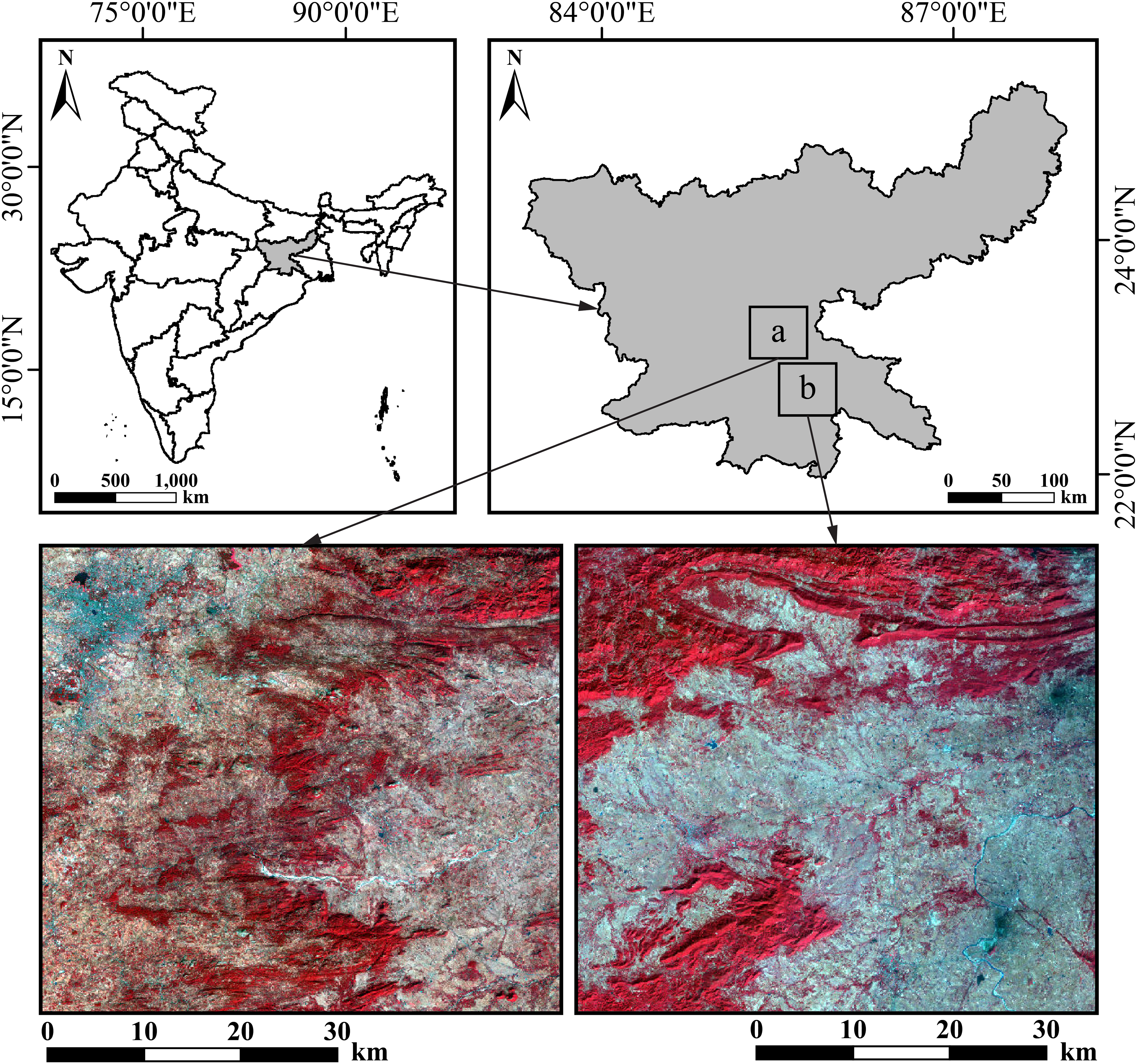
This study is based on two regions of interest in Jharkhand, India, here referred to as primary and secondary (Fig. 1). The primary region, with a geographical extent of 85° 15′ to 85° 45′ East and 22° 59′ to 23° 25′ North is used for the development of the LST downscaling methodology. This region is situated on the Ranchi plateau, the most extensive part of the Chota Nagpur Plateau. The region is an almost square patch of approximately 2,500 km2, partly overlapping with the city of Ranchi and includes the surrounding agricultural and forested areas, ensuring heterogeneity for model development. Its topography is characterized by plateaued, hilly upland terrain with an elevation above the mean sea level ranging from 151 to 780 m. The mean elevation is 416 m, indicating that a considerable proportion of the region is concentrated at higher altitudes. The dominant soil types are red and yellow soils (classified primarily as Alfisols and Inceptisols), formed from the underlying granite and gneiss bedrock, and are typically acidic with low to medium fertility (https://www.sameti.org/). The natural vegetation consists of tropical moist and dry deciduous forests, with sal (Shorea robusta), mahua (Madhuca longifolia), and palash (Butea monosperma) being the primary tree species (https://fsi.nic.in/forest-report-2021).
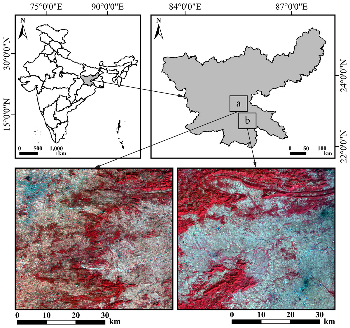
Figure 1: Study regions: (A) primary region where the RF, XGBoost and CatBoost models were trained, and (B) secondary region where these models were applied.
The secondary region is also an almost square patch of approximately 2,500 km2, with a geographical extent spanning 85°30′ to 85°59′ East and 22°30′ to 22°56′ North. It is a lower plateau with a more varied terrain of rolling plains and isolated hills. It is used to evaluate the predictive capability of the trained model developed using the primary region’s data. While it shares similar primary land cover types like forest land, cropland, and permanent waterbodies, it has a broader elevation range (87–863 m) and a lower mean elevation (242 m) compared to the primary region. Both study regions experience humid subtropical to tropical wet and dry climates, with temperatures soaring up to 45 °C in summer and dropping below 5 °C in winter. The southwest monsoon brings substantial rainfall, with an average annual precipitation ranging from 1,200 to 1,400 mm (Gupta, Banerjee & Gupta, 2021; Mahato et al., 2021). These study regions have been selected based on similar physical characteristics.
Datasets and methodology
The proposed methodology for downscaling MODIS LST incorporates a systematic workflow that combines a recursive feature elimination with cross-validation (RFECV) method to select relevant features, an ensemble machine learning model (RF), and multi-source data integration to enhance the spatial resolution of LST data acquired over six different dates (Table 1), representing six different months (January, February, May, June, November, and December). MODIS and Landsat 9 data were chosen from the exact dates across the six months to minimize bias in the dataset, except for 2022.11.12. Due to the absence of MODIS data over the regions of interest on 2022.11.12, the data from the subsequent day was incorporated into the model. This decision is supported after observing minimal meteorological variability in the parameters obtained from the ERA5-Land reanalysis dataset (https://doi.org/10.24381/cds.e2161bac) between the two dates, ensuring that the substitution does not introduce significant inconsistencies in the analyses. All product identifiers of the different datasets used in this study conform to the nomenclature established in the Earth Engine Data Catalog.
| Month | Landsat 9 OLI/TIRS-2 | MODIS | ||
|---|---|---|---|---|
| Date | Landsat 9 Product ID | Date | MOD09GA & MOD11A1 Product IDs | |
| January | 2022.01.28 | LANDSAT/LC09/C02/T1/LC09_140044_20220128 | 2022.01.28 | MODIS/061/MOD09GA/2022_01_28 |
| MODIS/061/MOD11A1/2022_01_28 | ||||
| February | 2022.02.13 | LANDSAT/LC09/C02/T1/LC09_140044_20220213 | 2022.02.13 | MODIS/061/MOD09GA/2022_02_13 |
| MODIS/061/MOD11A1/2022_02_13 | ||||
| May | 2022.05.20 | LANDSAT/LC09/C02/T1/LC09_140044_20220520 | 2022.05.20 | MODIS/061/MOD09GA/2022_05_20 |
| MODIS/061/MOD11A1/2022_05_20 | ||||
| June | 2022.06.05 | LANDSAT/LC09/C02/T1/LC09_140044_20220605 | 2022.06.05 | MODIS/061/MOD09GA/2022_06_05 |
| MODIS/061/MOD11A1/2022_06_05 | ||||
| November | 2022.11.12 | LANDSAT/LC09/C02/T1/LC09_140044_20221112 | 2022.11.13 | MODIS/061/MOD09GA/2022_11_13 |
| MODIS/061/MOD11A1/2022_11_13 | ||||
| December | 2022.12.14 | LANDSAT/LC09/C02/T1/LC09_140044_20221214 | 2022.12.14 | MODIS/061/MOD09GA/2022_12_14 |
| MODIS/061/MOD11A1/2022_12_14 | ||||
The independent variables in this study were derived from multiple satellite sensors. A summary of these datasets and their sources (sensors) is provided in Table 2. The satellite images from all the acquisitions were cloud-free, hence, no cloud-masking was done. “No data” values were absent in all the images, which avoided imputations and removal of pixels. Appropriate rescaling factors were used to convert the raw pixels into physical quantities (reflectance and temperature values). Normalization or standardization was not performed, as these are not prerequisites for an RF implementation. Each split within the decision trees is decided by simple threshold comparisons invariant to monotonic rescaling of individual variables.
| Dataset | Sensor | Platform | Spatial resolution | Temporal resolution | Swath |
|---|---|---|---|---|---|
| Land Surface Temperature (LST) | Moderate Resolution Imaging Spectroradiometer (MODIS) | Terra | 1 km | Daily | 2,330 km |
| Thermal Infrared Sensor-2 (TIRS-2) | Landsat 9 | 100 m (resampled to 30 m) | 16 days | 185 km | |
| Surface Reflectance | MODIS | Terra | 500 m | Daily | 2,330 km |
| Digital Elevation Model (DEM) | Panchromatic | Cartosat-1 | 30 m | 5 days (targeted revisit) | 26–30 km (stereoscopic) |
MODIS spectral bands and LST
MOD09GA.061 dataset (https://doi.org/10.5067/MODIS/MOD09GA.061) was used to select six spectral bands, namely blue, green, red, near infrared (NIR), shortwave infrared 1 (SWIR1), and shortwave infrared 2 (SWIR2). MOD11A1.061 dataset (https://doi.org/10.5067/MODIS/MOD11A1.061) was used to derive the LST. MODIS LST products store raw data as scaled integers to optimize storage efficiency and maintain precision. A scaling factor of 0.02 is applied to convert these integer values into physically meaningful LST values in Kelvin (K). Finally, temperatures in degrees Celsius (°C) are derived by subtracting 273.15 from the Kelvin results.
MODIS vegetation indices
The MOD09GA.061 dataset was used to derive the following vegetation indices:
Normalized difference vegetation index
(1)
Normalized difference water index
(2)
Modified normalized difference water index
(3)
Normalized difference built-up index
(4)
Soil-adjusted vegetation index
(5)
Here, is the soil brightness correction factor.
Vegetation indices are integral to LST downscaling as they provide essential information about vegetation cover, influencing surface temperatures (Wang et al., 2021; Pandey et al., 2023).
For digital elevation model data, two scene IDs, P5_PAN_CS_N22_000_E085_000_30m and P5_PAN_CS_N23_000_E085_000_30m from the PAN sensor of the CartoSat-1 satellite (https://bhoonidhi.nrsc.gov.in/bhoonidhi/index.html) were mosaiced to encompass the regions of interest.
Landsat 9 LST retrieval
The NDVI threshold-based emissivity method is one of the approaches to retrieve Landsat 9 LST.
The raw sensor-specific quantized and calibrated digital numbers (DNs) stored in Landsat imagery (https://earthexplorer.usgs.gov/) are converted into physically quantifiable radiance units.
(6) Here, and are the band-specific multiplicative (gain) and additive (offset) rescaling factors, respectively, provided in the imagery’s metadata file, and denotes the quantized and calibrated pixel values (DNs).
The inverse of Planck’s function is applied to convert radiance into brightness temperature.
(7) Here, and are band-specific thermal conversion constants extracted from the metadata, and is the spectral radiance in .
To adjust the brightness temperature for actual surfaces, each pixel’s surface emittance of thermal radiation is considered. The emissivity depends on surface composition, as vegetation, soil, rock, water, and urban infrastructure emit radiation differently. To quantify this, is computed. The following equation calculates the proportion of vegetation, within a pixel, representing the extent of green vegetation cover to quantify surface heterogeneity, using NDVI extremes for “complete vegetation” ( ) and “bare soil” ( ).
(8) Higher vegetation cover has higher emissivity, while bare soil or rock has lower emissivity. Using and known emissivity values for dense vegetation and bare soil, land surface emissivity (LSE) for each pixel is dynamically calculated using Eq. (9).
(9) Here, and are the emissivities of bare soil and pure vegetation, respectively, and represents surface roughness, taken as a constant.
Empirical NDVI-based emissivity relationships have been used extensively in the literature. These methods ensure that LSE is not treated as a constant but is spatially dynamic and tailored to the surface conditions (Sobrino, Jiménez-Muñoz & Paolini, 2004; Momeni & Saradjian, 2007; Sobrino et al., 2008; Li et al., 2013). For a smooth transition, emissivity was modeled as ε = 0.004Pv + 0.986 in this study.
With LSE determined, the at-sensor brightness temperature is converted to LST by accounting for the reduced recorded thermal radiance caused by the surface’s deviation from an ideal blackbody behavior.
(10) Here, is the brightness temperature, is the center wavelength of the TIR band (band 10) in , and is derived from Eq. (11), and is the LSE.
(11) Here, is the Planck’s constant ( ), σ is the Boltzmann constant ( ), and is the velocity of light ( ).
Model construction using RF
The RF model is a powerful ensemble machine-learning method introduced by Breiman (2001). It is a low-bias, low-variance model as it tends to generalize well and perform consistently across training and test datasets. RF effectively handles large datasets that exhibit complex relationships. It is capable of noise reduction and outlier removal, and avoids overfitting problems by averaging the outputs of many decorrelated trees (Prasad et al., 2020; Njuki, Mannaerts & Su, 2020). The decorrelation is achieved through bootstrapping and selecting a random subset of features at each split. The interpretability through feature importance is a significant advantage.
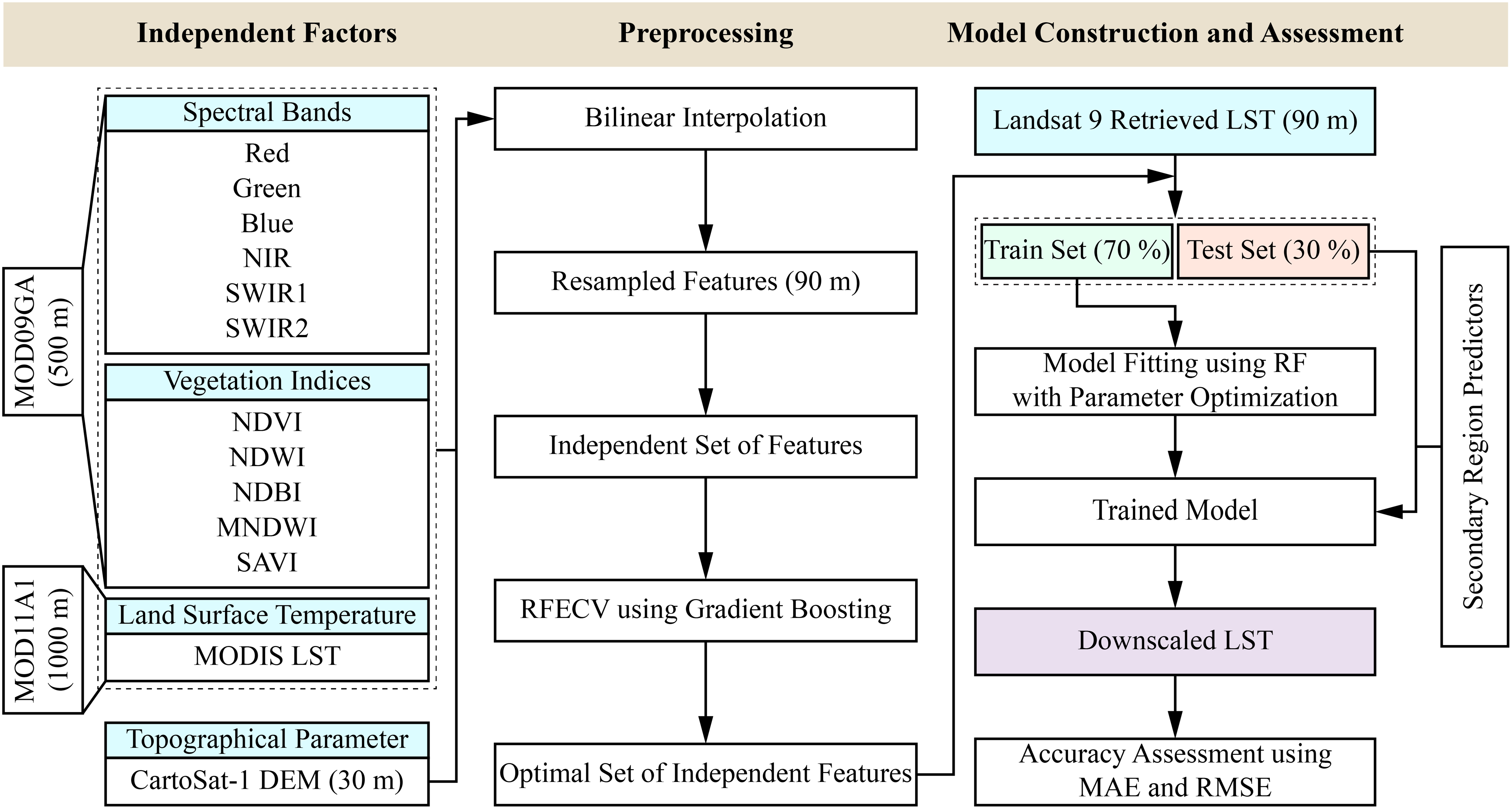
There are different feature selection methods, namely Boruta, RFE, and multicollinearity methods, which have been applied in various studies (Prasad et al., 2023; Abdo et al., 2024). This study initially considered thirteen independent features for the primary region. To mitigate the curse of dimensionality and prevent overfitting, an RFECV method using gradient boosting was employed, selecting eight relevant independent features to enhance the model’s generalization capability (Barzani et al., 2024). The eight features include four spectral bands (blue, near infrared (NIR), shortwave infrared (SWIR)1, and SWIR2), two vegetation indices (MNDWI and SAVI), MODIS LST, and digital elevation model (DEM) processed from two CartoSat-1 scenes as the only topographic feature. Finer resolution (90 m) Landsat 9-retrieved LST was used as the target variable. The 90-m scale was fixed to preserve the band’s native resolution maximally. The Landsat LST data was processed and directly exported to a 90-m scale in Google Earth Engine (GEE). All the MODIS variables and DEM were resampled to 90 m using bilinear interpolation for spatial congruence with the target variable.
The model (Fig. 2) was built using optimal parameters obtained after randomly exploring 50 combinations from the grid of values of five parameters (Table 3), namely n_estimators, criterion, max_depth, min_samples_leaf, and max_features, with a 5-fold cross-validation using the RandomizedSearchCV method of the open-source scikit-learn Python library to minimize the bias-variance trade-off for improving the model’s predictive accuracy and achieve robustness (Bergstra & Bengio, 2012). The minimum value in the set of values for min_samples_leaf was carefully chosen to be 10 to restrain the growth of the decision trees to the deepest level, avoiding the risk of fitting any potential outliers. The parameter n_jobs was set to −1 to involve all the CPU cores for parallelization. The RandomizedSearchCV method was employed to reduce computational time while exploring diverse combinations. All the computing was done by an AMD Ryzen 5 5600H processor (3.30 GHz) with 16 GB RAM (3,200 MHz) in a Windows 11 environment.
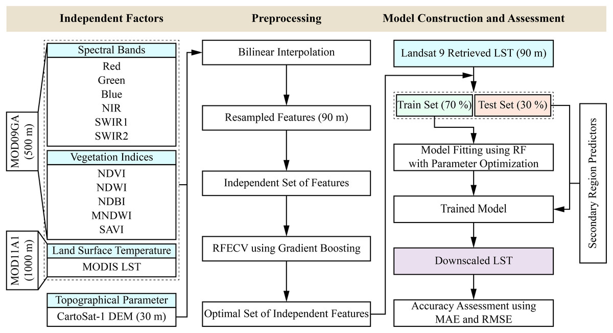
Figure 2: Flow diagram of the downscaling methodology.
| Scikit-learn parameter | Description | Values | Optimal value |
|---|---|---|---|
| n_estimators | The number of decision trees | [50, 70, 100] | 100 |
| criterion | The function to measure the quality of a split | [‘squared_error’, ‘friedman_mse’] | ‘friedman_mse’ |
| max_depth | The maximum depth of a decision tree | [25, 30, 35, None] | None |
| min_samples_leaf | The minimum number of samples required to be at a leaf node | [10, 15, 20] | 10 |
| max_features | The subset of features considered for each split | [‘sqrt’, ‘log2’, None] | None |
To evaluate the model’s generalization capability and avoid overfitting, the dataset was partitioned into training and test subsets in the ratio 7:3, ensuring the model was validated on unseen data before applying it to the secondary region. Once trained, the RF model was used to predict the LST for the secondary region, enhancing the spatial resolution of the MODIS LST. The following metrics (Eqs. (12)–(14)) were used to evaluate the downscaling performance of the RF regression model for both the primary and secondary regions. Since the model was trained on 70% of the data from the primary region, the remaining 30% was used to evaluate the model to obtain an unbiased estimate of its predictive performance. The trained model was then applied to the secondary region for the reproducibility of similar results observed in the primary region’s test set.
(12)
(13) Here, and are actual and predicted LST values for -th pixel, respectively, and is the number of pixels.
(14) Here, is the mean around the actual LST values, and is the number of pixels.
Results
Feature importance by RF
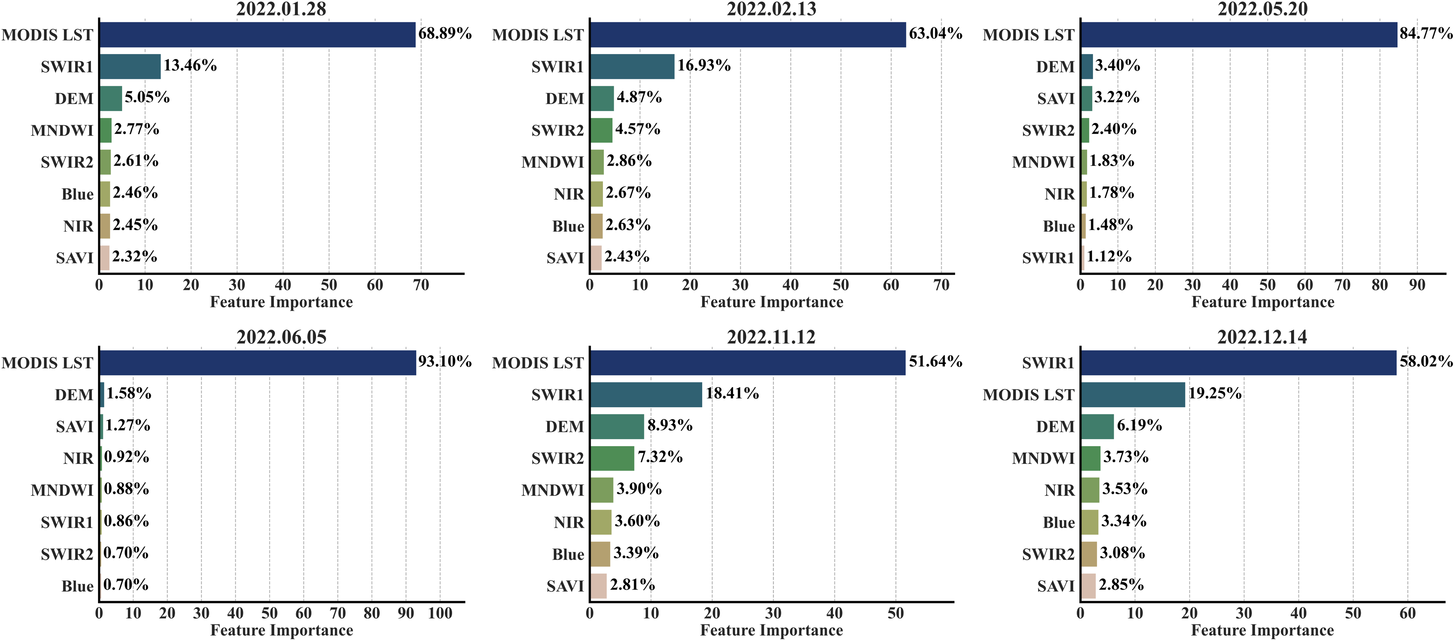
Determining the importance of features is essential in LST, natural resources, and hazard mapping (Prasad et al., 2022, 2024, 2025). The feature importance plots of the primary region (Fig. 3) weigh heavily on three factors, namely, SWIR1, MODIS LST, and DEM. MODIS LST contributed 68.89% and 63.04% in January and February, respectively, to the model’s predictions. In these months, SWIR1 was the next highest contributor, influencing the predictions by 13.46% and 16.93%, respectively. The influence of MODIS LST in May and June elevated to 84.77% and 93.10%, respectively, undermining all other features. A contrasting dynamic was observed in December, where the importance of SWIR1 dominated all other features, influencing 58.02% of the model’s predictions. There are notable spikes in the importance of the other factors, namely NIR, blue, SWIR2, SAVI, MNDWI, and DEM, in November compared to January, February, May, and June. The most important feature for spatial downscaling was MODIS LST, followed by SWIR1, DEM, SWIR2, and MNDWI. In contrast, the blue band, SAVI, and NIR band were among the less important factors.
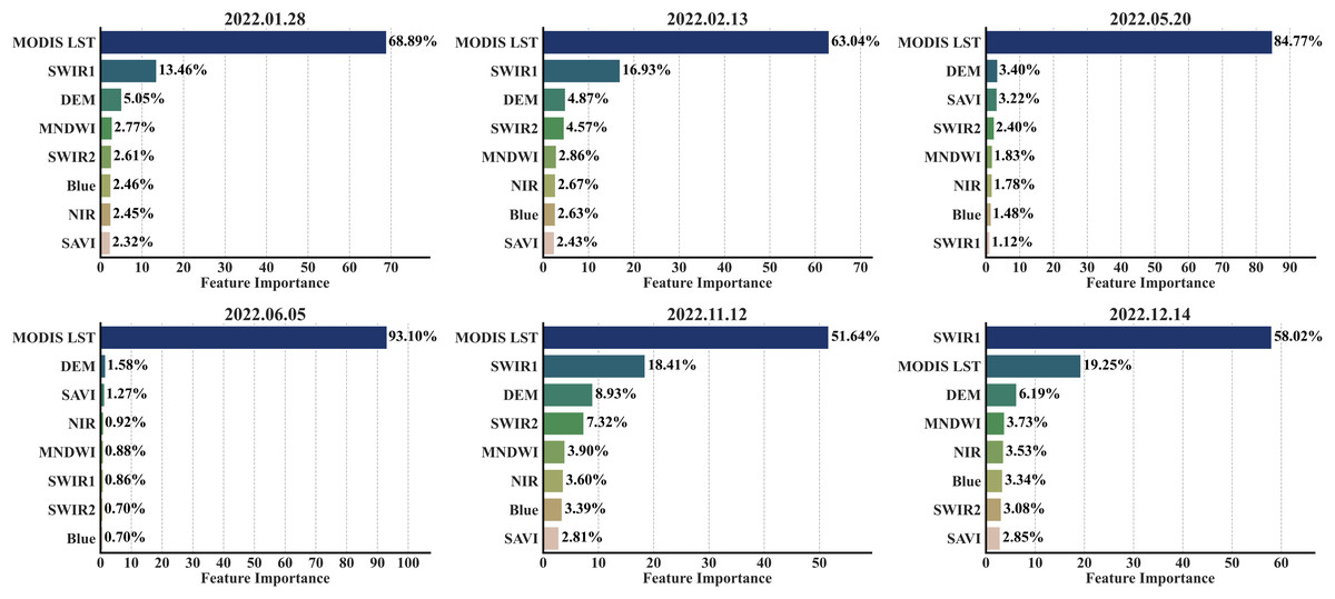
Figure 3: RF importance scores across all acquisition dates.
Downscaling performance
The predictions on the test data across all the months aligned closely with the actual LST values (Table 4). The mean temperatures were consistent, with trifling deviations in the months of February and December. The model performed exceptionally well in May and June, as evident by the root mean square error (RMSE) and R2 values. In June, the RMSE was the lowest, and the R2 value maximally justified the 1:1 ideal line, explaining 96% of the variability. The spread of LST values, reflecting the level of information acquired (Mukherjee, Joshi & Garg, 2017; Maithani et al., 2022), was significantly closer to the actual variance in June. The model predicted a variance of 6.83 against the actual 7.25. This month’s minimum and maximum predicted LST values of 27.10 °C and 40.30 °C depicted the closest resemblance to the actual LST range, justifying the actual variance. The predictions were weaker in the months of February and December, with lower variances. The R2 was relatively lower (0.76) in November and December, indicating the model’s inefficiency in fully capturing the variability. The test predictions also revealed a general tendency to compress the maximum and marginally elevate the minimum temperatures, affecting the variability. Substantial compression in the temperature ranges can be observed in the months of February and November, with deviations of 3.56 °C and 3.50 °C. The model’s tendency to underestimate high temperatures is offset by its simultaneous overestimation of low temperatures, keeping the mean temperatures consistent with the actual values. This predictive behavior is a fundamental characteristic of RF regression and is attributed to the model’s approach to averaging the outputs from all the decision trees.
| Month | Date | LST | Min | Max | Mean | Variance | MAE | RMSE | R2 |
|---|---|---|---|---|---|---|---|---|---|
| January | 2022.01.28 | Actual | 12.11 | 24.03 | 17.76 | 1.64 | 0.41 | 0.56 | 0.81 |
| Predicted | 12.51 | 22.52 | 17.76 | 1.23 | |||||
| February | 2022.02.13 | Actual | 16.53 | 30.74 | 23.11 | 2.70 | 0.57 | 0.76 | 0.79 |
| Predicted | 17.37 | 28.02 | 23.12 | 1.98 | |||||
| May | 2022.05.20 | Actual | 27.29 | 44.19 | 37.58 | 4.74 | 0.48 | 0.65 | 0.91 |
| Predicted | 27.41 | 41.99 | 37.58 | 4.15 | |||||
| June | 2022.06.05 | Actual | 26.60 | 41.30 | 33.68 | 7.25 | 0.39 | 0.54 | 0.96 |
| Predicted | 27.10 | 40.30 | 33.68 | 6.83 | |||||
| November | 2022.11.12 | Actual | 20.61 | 34.39 | 25.53 | 1.94 | 0.52 | 0.68 | 0.76 |
| Predicted | 20.83 | 31.11 | 25.53 | 1.33 | |||||
| December | 2022.12.14 | Actual | 18.03 | 32.30 | 23.24 | 2.14 | 0.55 | 0.72 | 0.76 |
| Predicted | 18.34 | 28.95 | 23.25 | 1.47 |
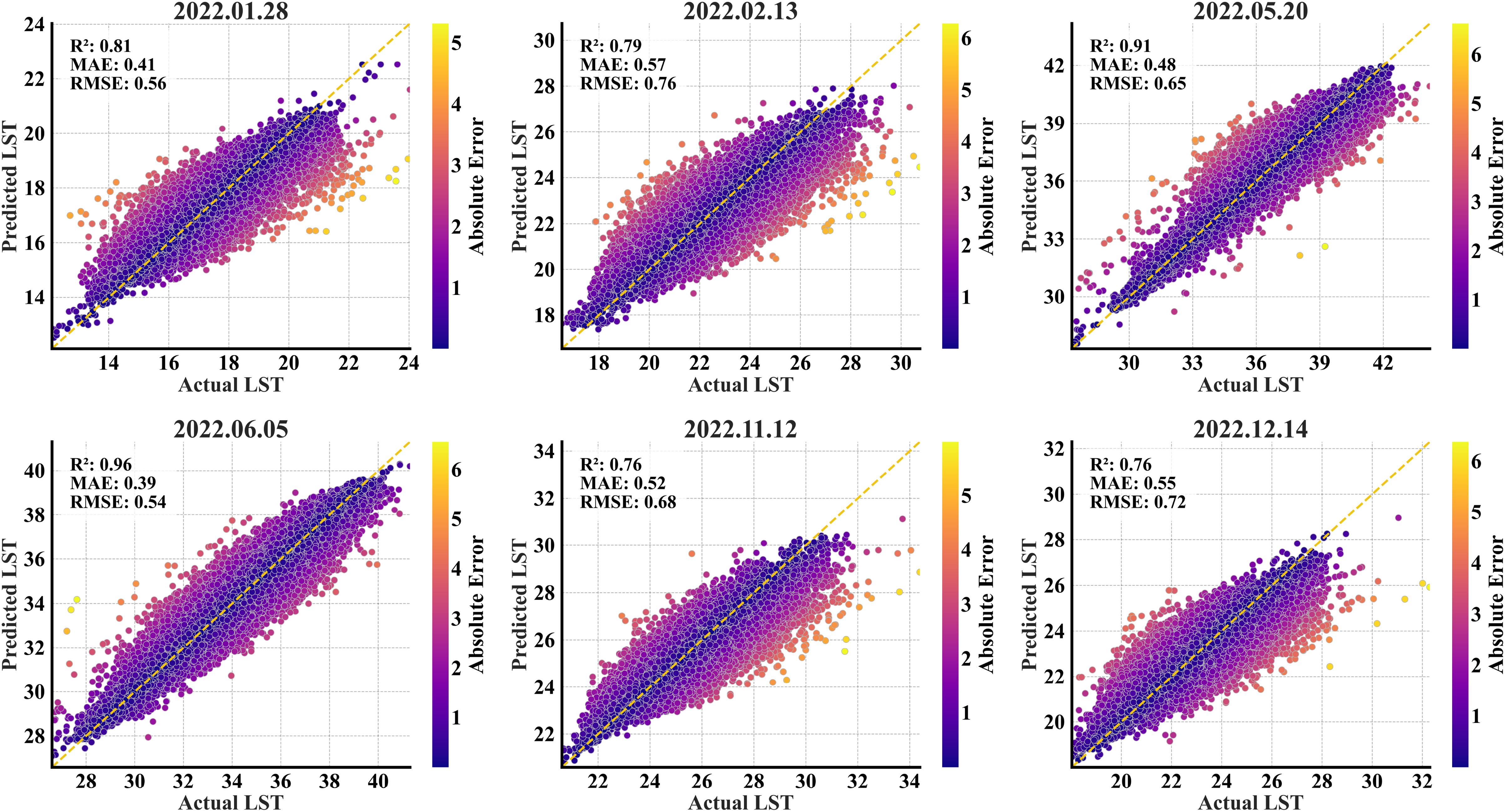
The scatterplots revealed a substantial concentration of predictions against the actual LST values on the 1:1 ideal line (Fig. 4). The model underestimated the higher temperatures in all the months except May and June. There was no considerable disarray of predictions in May and June, and a small number of predictions were affected by a high error magnitude. Overall, the magnitude of errors was relatively greater on the edges of the actual temperature spectrum across all the months.
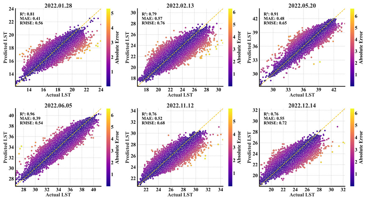
Figure 4: RF scatterplots of the predicted refined LST (y-axis) vs. actual Landsat 9 LST (x-axis) data at 90 m for the primary region’s test set; the yellow dashed diagonal line represents the 1:1 ideal line.
The error histograms exhibited the model’s unbiased predictability, as the errors were symmetrically distributed around zero for all the months (Fig. 5). The bell-shaped curves suggest a normal distribution of errors, with most errors accumulating within the range of −2 to +2 °C. A high percentage of errors has a ±1 °C offset from the ideal value of 0 across all the months. The narrower distributions in May and June, particularly June, highlighted the model’s strong performance with fewer errors and more accurate predictions.
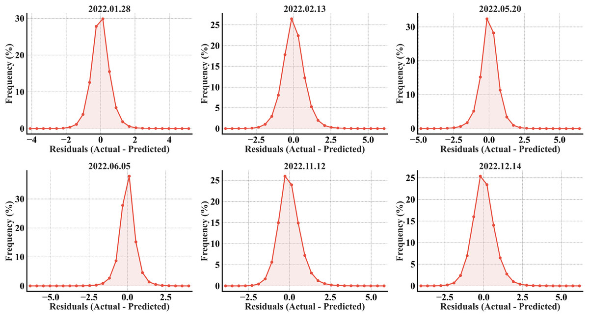
Figure 5: RF error histograms from the predicted refined LST across all acquisition dates for the primary region’s test set; the x-axis represents the prediction error in °C, and the y-axis represents the percentage of total pixels.
Model transferability
The trained RF model was applied to the secondary region to assess its transferability. It showed a moderate drop in efficiency, reflecting the challenges of applying models to unknown spatial contexts. The secondary region analyses yielded R2 values between 0.65 and 0.76, with RMSE values ranging from 0.85 °C to 1.18 °C (Table 5). The predictions in January had an RMSE of 1.01 and an R2 of 0.76. The variability was underrepresented in the predicted temperatures, with the predicted variance (2.87) lower than the actual variance (4.22). A similar pattern was observed in February with an RMSE of 0.96 and an R2 of 0.74. The predicted mean LST (22.34 °C) closely matched the actual mean (22.36 °C). Contrary to the test results, the model’s performance declined considerably in May and June in the secondary region with RMSEs of 1.18 and 1.01, respectively. The lower R2 values indicated a weaker alignment of predictions against the actual values. With an RMSE of 0.85 and an R2 value of 0.74, the November predictions captured trends to a large extent and maintained variability. In December, the model yielded an RMSE of 1.12 and an R2 of 0.73. The predicted variance (3.10) in this month was significantly lower than the actual variance (4.74), reflecting limitations in capturing local variability. The model’s performance in simulating the temperature ranges varied seasonally within the secondary region. While the model depicted fair agreement with the observed temperature ranges during the peak warm months (especially the month of May), it consistently underestimated the temperature variations in the transitional months (January, February, November, and December), mostly estimating narrower ranges than observed.
| Month | Date | LST | Min | Max | Mean | Variance | MAE | RMSE | R2 |
|---|---|---|---|---|---|---|---|---|---|
| January | 28.01.2022 | Actual | 11.28 | 27.65 | 18.72 | 4.22 | 0.82 | 1.01 | 0.76 |
| Predicted | 12.49 | 20.84 | 18.17 | 2.87 | |||||
| February | 13.02.2022 | Actual | 15.31 | 31.24 | 22.36 | 3.57 | 0.73 | 0.96 | 0.74 |
| Predicted | 17.34 | 26.66 | 22.34 | 3.13 | |||||
| May | 20.05.2022 | Actual | 29.13 | 43.05 | 36.46 | 4.60 | 0.92 | 1.18 | 0.69 |
| Predicted | 28.20 | 41.63 | 36.63 | 4.36 | |||||
| June | 05.06.2022 | Actual | 24.70 | 37.28 | 30.05 | 2.92 | 0.81 | 1.01 | 0.65 |
| Predicted | 27.79 | 35.83 | 30.50 | 2.15 | |||||
| November | 12.11.2022 | Actual | 19.49 | 35.77 | 25.49 | 2.76 | 0.66 | 0.85 | 0.74 |
| Predicted | 21.00 | 29.74 | 25.51 | 2.44 | |||||
| December | 14.12.2022 | Actual | 16.70 | 31.51 | 23.29 | 4.74 | 0.86 | 1.12 | 0.73 |
| Predicted | 18.36 | 27.09 | 23.08 | 3.10 |
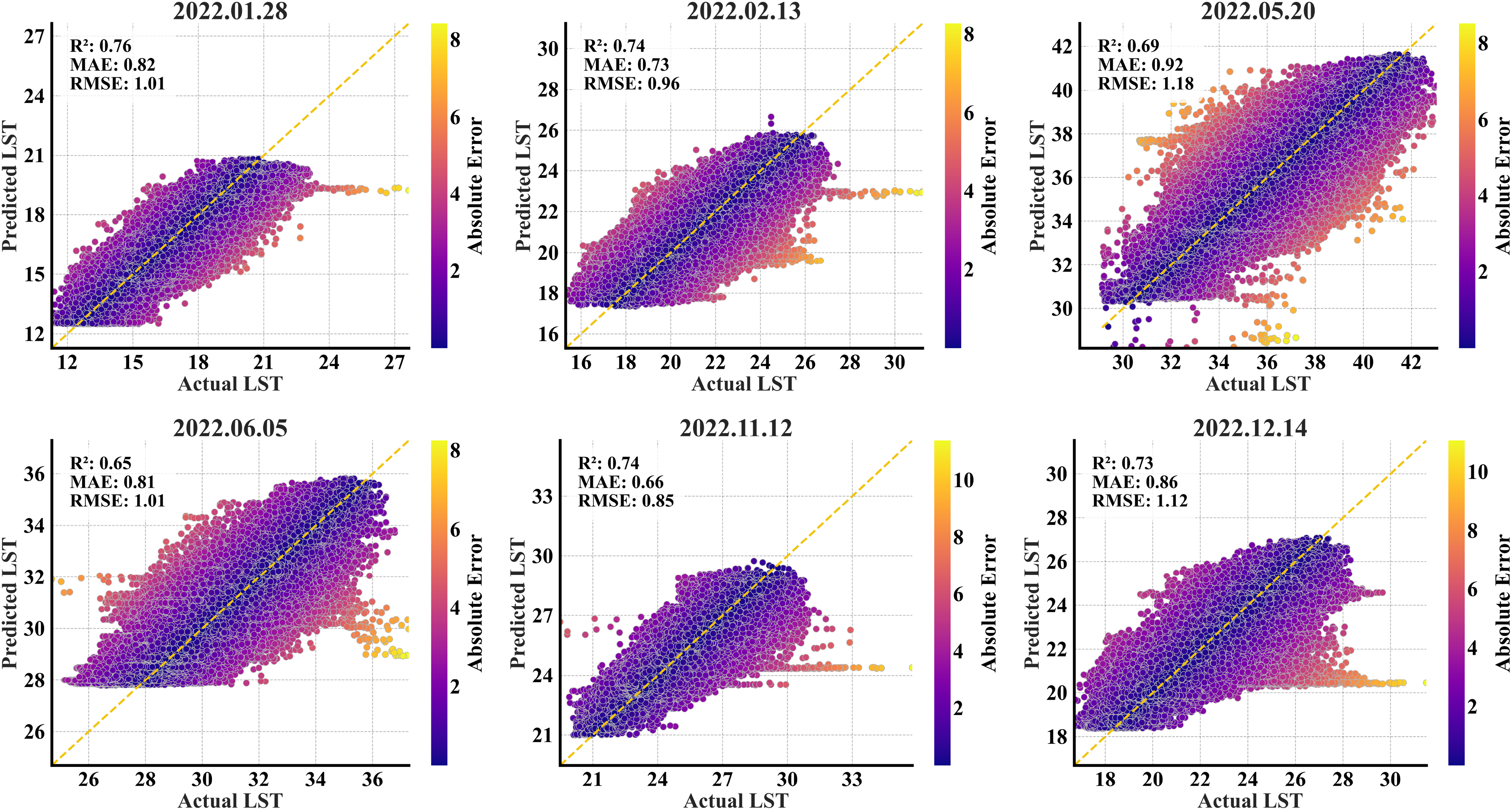
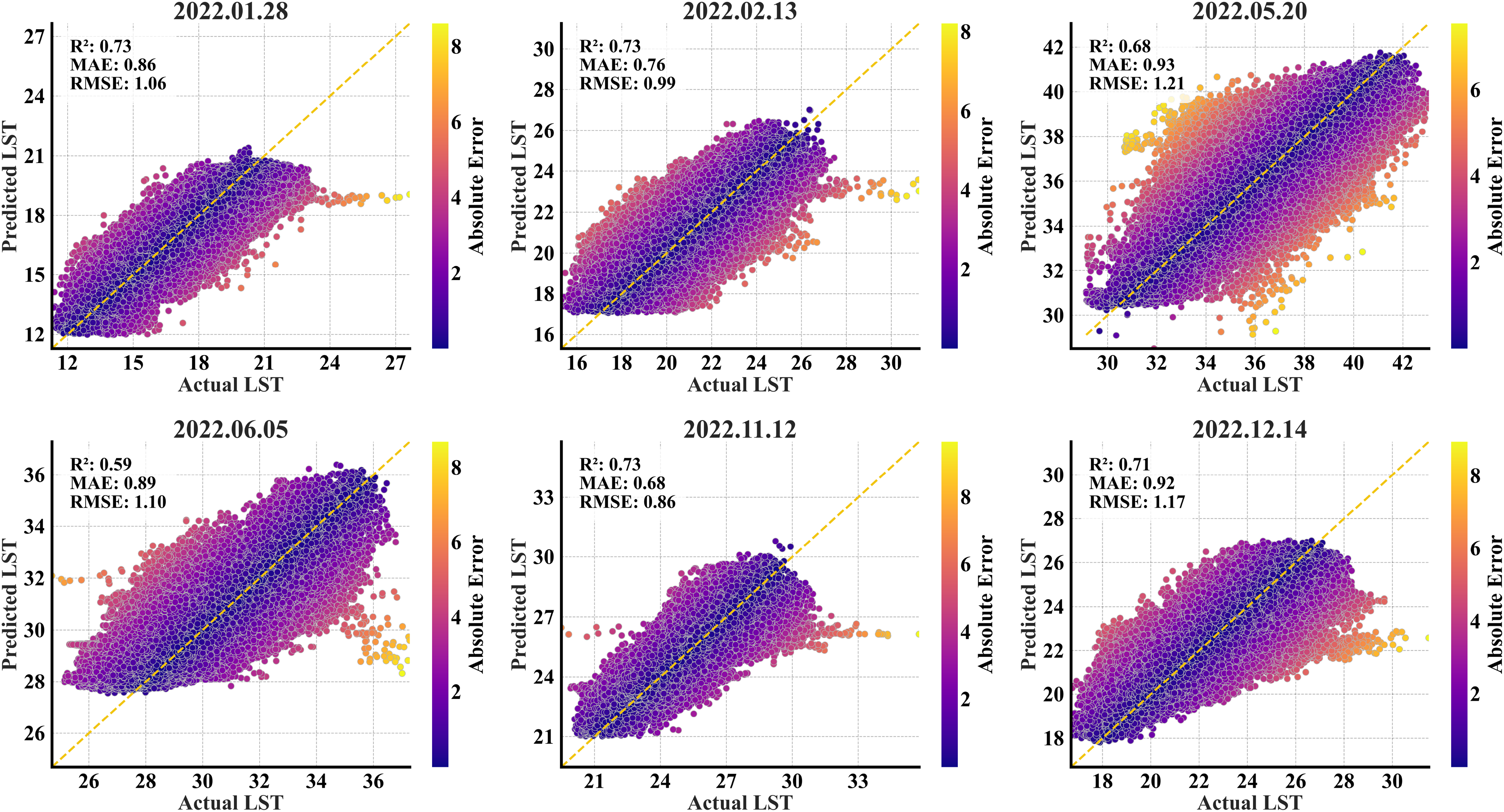
The secondary region scatterplots (Fig. 6) showed a derangement of some predictions, suggesting weaker correlations in all the months, notably the May and June months. There is a consistent underestimation of higher temperature ranges in all the months. While most predictions are tightly clustered along the 1:1 ideal line, indicating smaller errors, larger errors tend to cluster at the extremes of the target range, suggesting the model’s sensitivity in predicting extreme values. Since the model was trained in the primary region, the clusters of incorrectly predicted points in these plots indicate that the secondary region exhibits different spatial features that were never represented in the training data. Despite variations in R2 values, the model maintained consistent performance throughout the six temporal points, never dropping below 0.65, suggesting fundamental reliability.
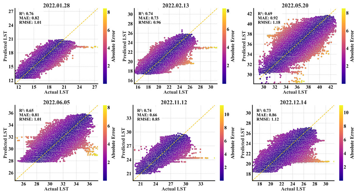
Figure 6: RF scatterplots of the predicted refined LST (y-axis) vs. actual Landsat 9 LST (x-axis) data at 90 m for the secondary region; the yellow dashed diagonal line represents the 1:1 ideal line.
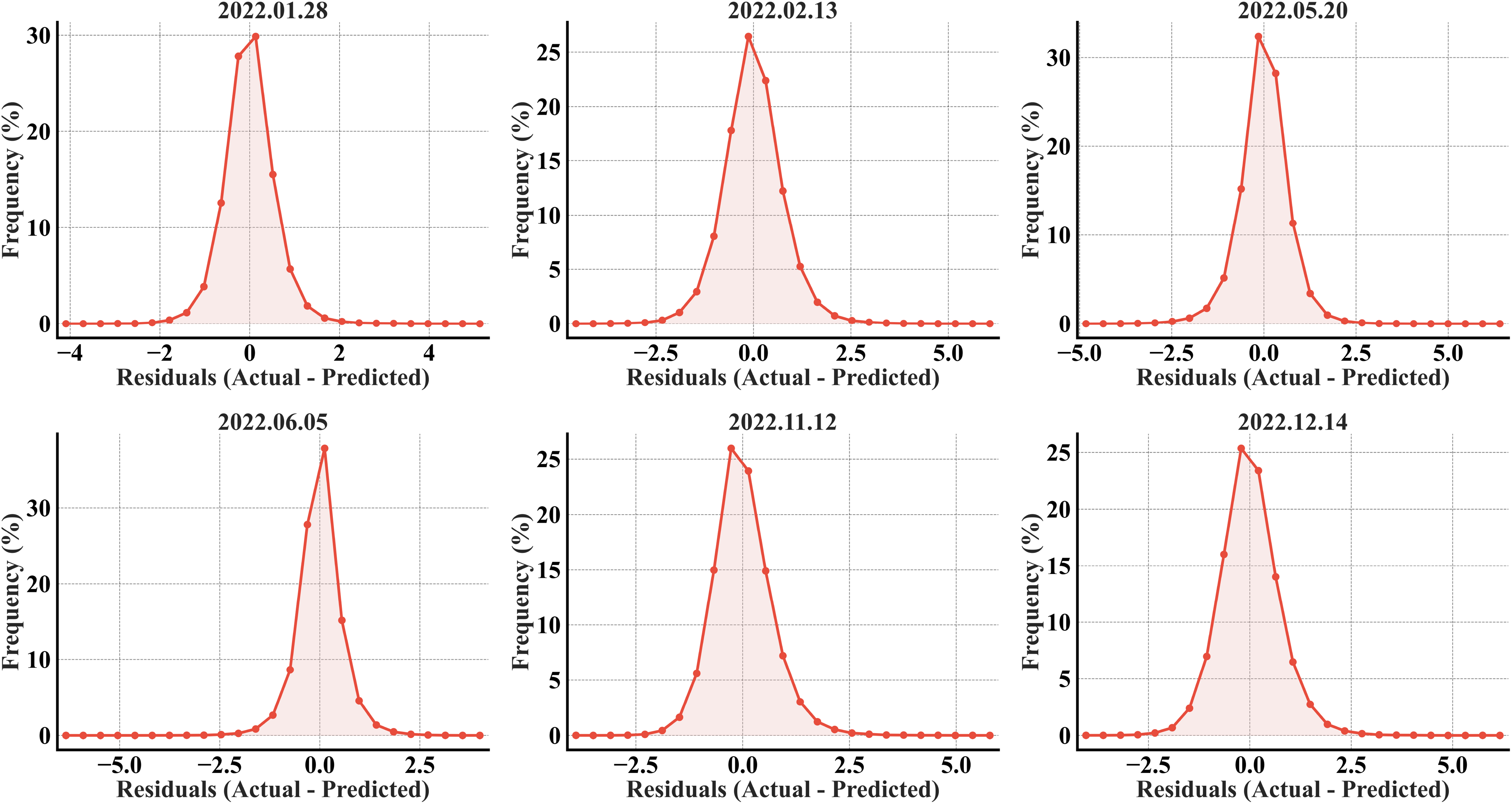
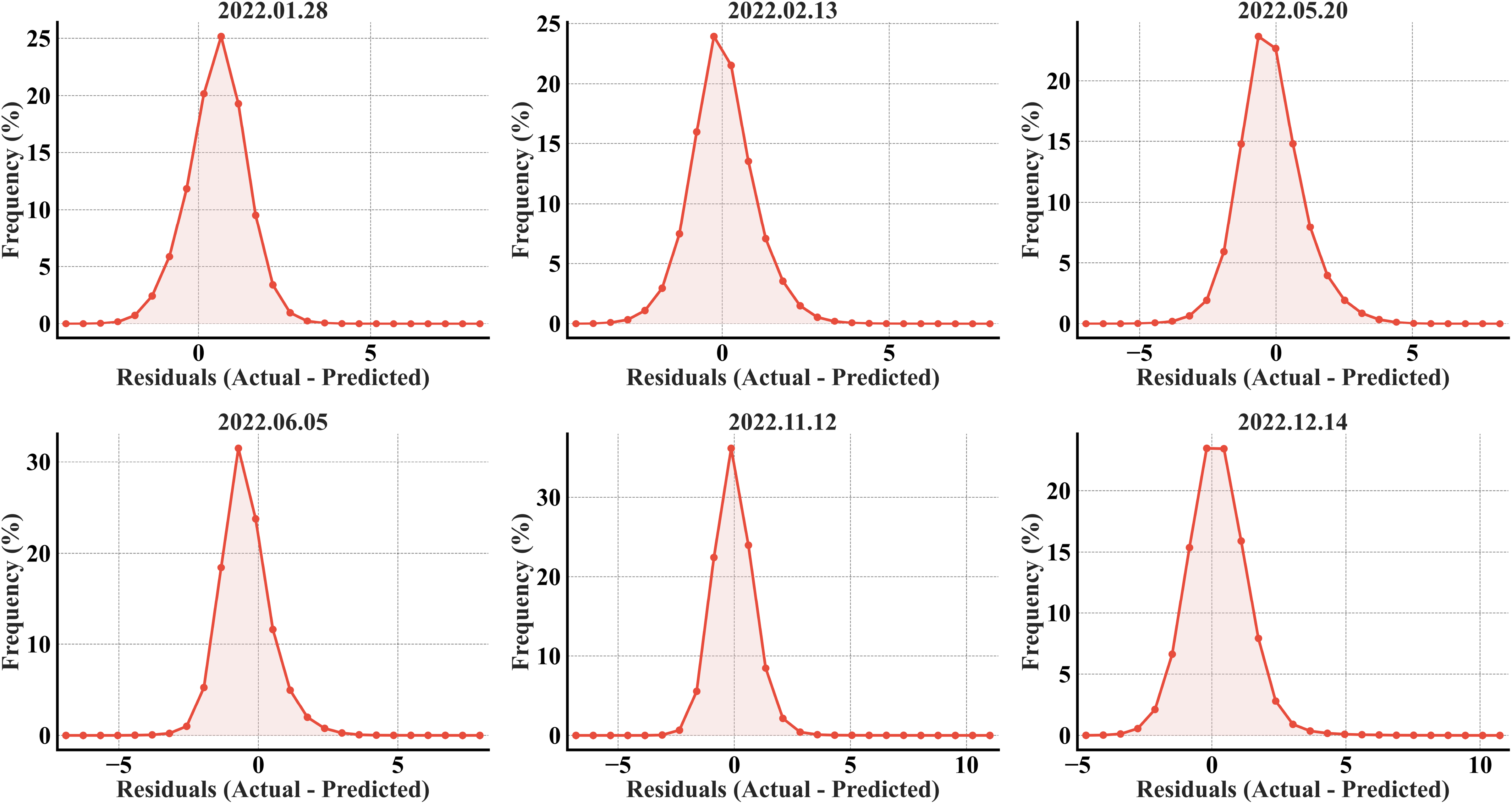
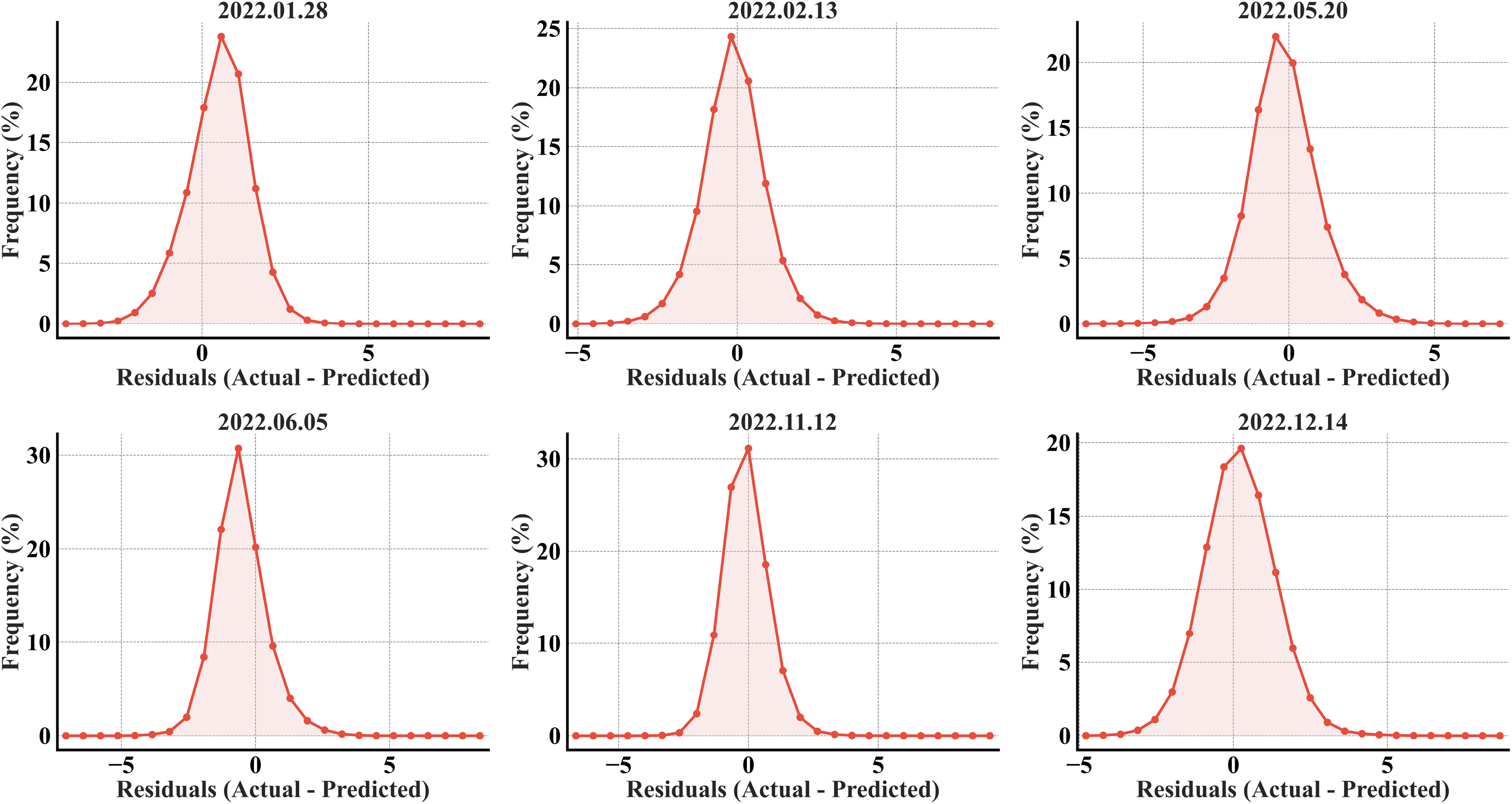
All six error histograms (Fig. 7) show a single, sharply peaked (high kurtosis) distribution around zero, especially in February, November, and December, indicating that most predictions align with the actual values. A slight offset in all the plots, evident from the right elongated tails in the distributions, further validates the underestimation in the predictions. The tails beyond ±2 °C for all the months confirm the existence of larger errors, but the rapid drop-off in frequency indicates they are relatively rare compared to the strong concentrations near zero.
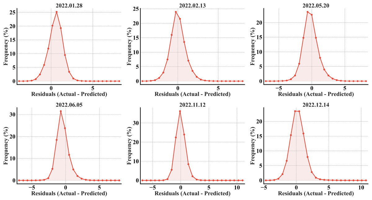
Figure 7: RF error histograms from the predicted refined LST across all acquisition dates for the secondary region; the x-axis represents the prediction error in °C, and the y-axis represents the percentage of total pixels.
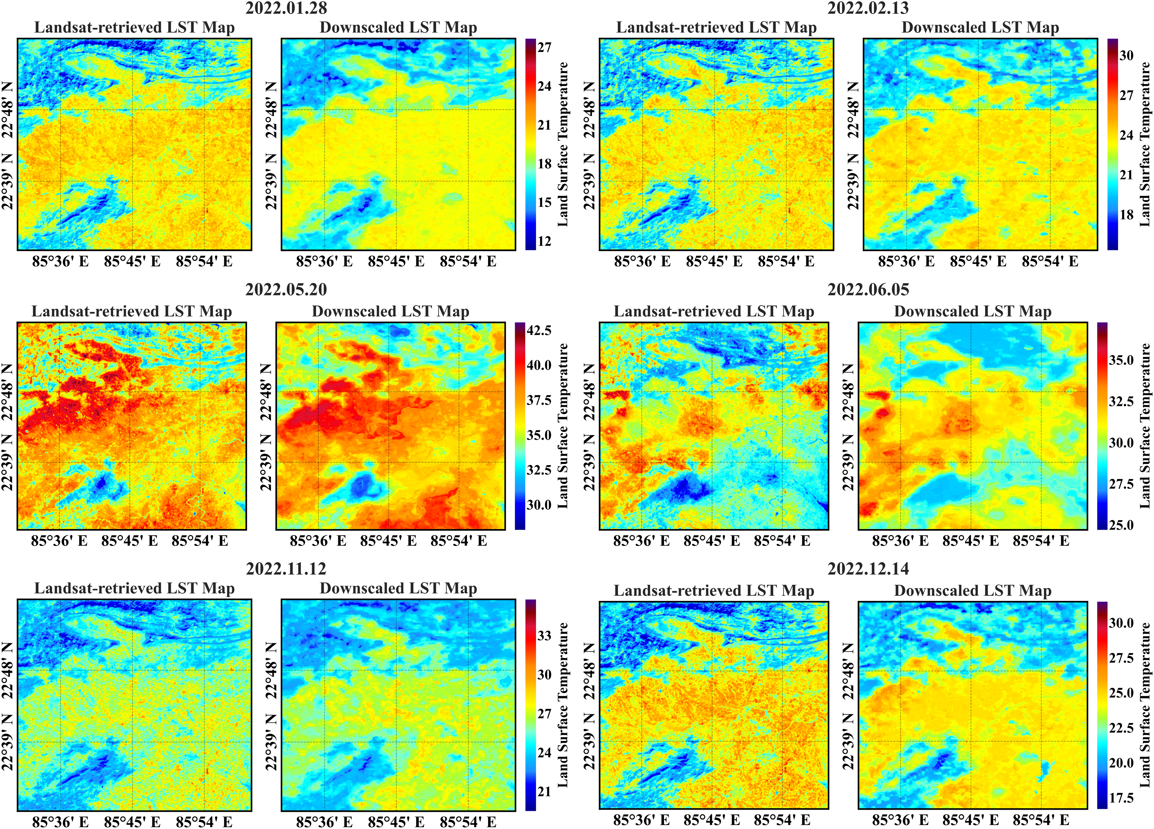
The secondary region’s actual and predicted 90-m LST maps are presented in Fig. 8. The temperature spectrum is represented in a color gradient from blue to red, with blue indicating lower temperatures and red indicating higher temperatures. A visual comparative analysis of the maps depicts considerable similarity, making the RF model suitable for downscaling.
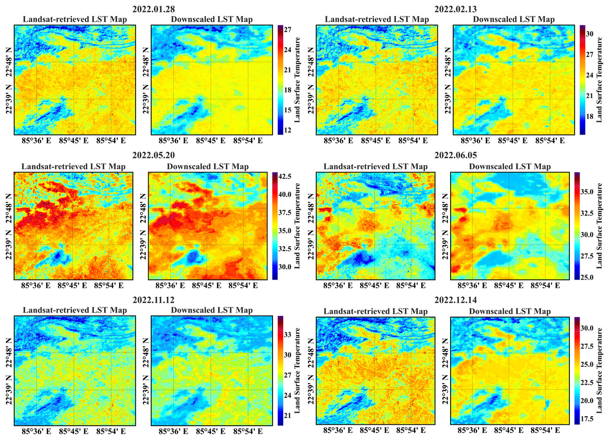
Figure 8: Actual vs. predicted 90 m LST maps of the secondary region from the RF model.
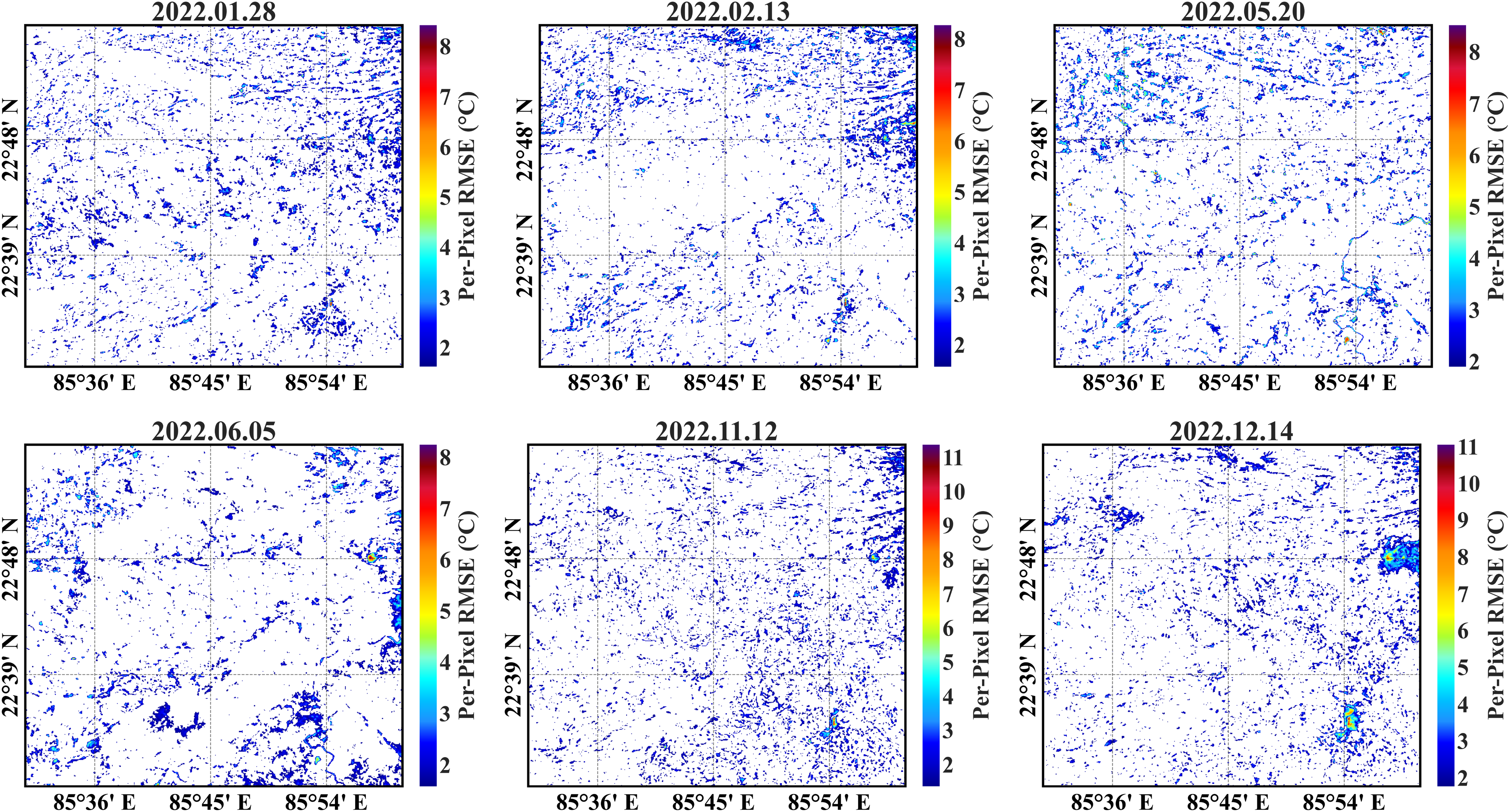
The considerable white sparse areas in the predicted per-pixel RMSE maps (Fig. 9) depict close alignment with the actual LST values with lesser deviation (≤1 °C). Most predictions can be observed within a derangement of 2 °C, with a significantly low number of predicted temperature values exceeding an RMSE beyond 3 °C.
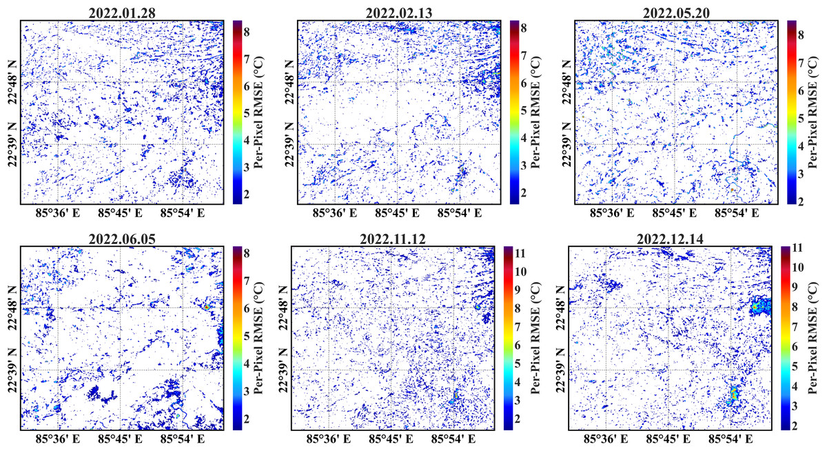
Figure 9: Per-pixel RMSE maps of the secondary region from the RF model; the white sparse areas have RMSE values less than 1 °C.
Comparative evaluation of RF against XGBoost and CatBoost
To contextualize the performance of the RF model, a comparative analysis was done using XGBoost and categorical boosting (CatBoost). These models were trained and evaluated using the exact temporal points, feature sets, datasets, and validation procedures to ensure an appropriate comparison of their downscaling capabilities.
The XGBoost model, introduced by Chen & Guestrin (2016), mitigates the common overfitting issue in traditional boosting models by incorporating regularization techniques. These penalties help control model complexity, preventing overfitting. The model’s objective function is optimized using a second-order Taylor expansion for faster convergence.
In the context of regression, CatBoost, introduced by Prokhorenkova et al. (2018) is a powerful gradient boosting algorithm that predicts a continuous target variable by minimizing the default RMSE loss function. CatBoost trains each tree on a sequence of randomly shuffled datasets, ensuring that the error for a particular data point is evaluated on a model that has not been trained on that specific data point. This leads to more robust models that generalize better to unseen data.
To ensure optimal performance, hyperparameter tuning was employed for both algorithms using a grid search strategy similar to the RF-based methodology. The number of different hyperparameter combinations (n_iter) was set to 50, keeping it consistent with the RF model. Tables 6 and 7 specify the relevant parameters that were tuned with the grid of values and the optimal combinations.
| Scikit-learn parameter | Description | Values | Optimal value |
|---|---|---|---|
| n_estimators | The total number of trees to build | [100, 200, 500, 1,000] | 500 |
| max_depth | The deepest a single tree can grow | [3, 5, 7, 9] | 9 |
| learning_rate | How much to shrink the contribution of each new tree | [0.01, 0.05, 0.1, 0.2] | 0.1 |
| subsample | The fraction of training data (rows) used for each tree | [0.7, 0.8, 0.9] | 0.8 |
| colsample_bytree | The fraction of features (columns) used for each tree | [0.8, 0.9, 1] | 1 |
| gamma | The minimum loss reduction needed to split a node further | [0, 0.1, 0.3, 0.5, 1] | 0.1 |
| min_child_weight | The minimum amount of data required in a new node | [1, 2, 3, 5, 10] | 3 |
| reg_lambda | The L2 regularization strength to prevent overfitting | [0.1, 1, 5, 10, 20] | 10 |
| Scikit-learn parameter | Description | Values | Optimal value |
|---|---|---|---|
| iterations | The maximum number of decision trees to build | [100, 200, 300, 500, 1,000] | 300 |
| depth | The maximum depth of each tree | [6, 8, 10, 12] | 12 |
| learning_rate | This scales the contribution of each tree | [0.01, 0.03, 0.05, 0.1] | 0.1 |
| l2_leaf_reg | The L2 regularization coefficient | [1, 3, 5, 10] | 1 |
| subsample | The fraction of training data (rows) sampled for each tree | [0.6, 0.8, 0.9, 1] | 1 |
| rsm | The proportion of features (columns) randomly selected for each tree | [0.7, 0.8, 0.9, 1] | 1 |
| bagging_temperature | Controls the intensity of bagging | [0, 0.5, 1, 2] | 0 |
The performance statistics for both primary and secondary regions are specified in Tables 8 and 9. The XGBoost model produced a performance profile highly similar to the RF model on the primary region’s test set (Table 8). Across all the months, the metrics for both models were almost identical, suggesting that XGBoost is an equally feasible model for this dataset, offering a similar predictive advantage. However, in the secondary region, it consistently underperformed compared to RF (Table 9). XGBoost registered a higher RMSE and a lower R2 value than the RF model across all six temporal points (Fig. 10). This suggests that the XGBoost model was slightly more biased to the primary region’s data and therefore less generalizable than RF.
| eXtreme gradient boosting | Categorical boosting | |||||||||||||||
|---|---|---|---|---|---|---|---|---|---|---|---|---|---|---|---|---|
| Min | Max | Mean | Variance | MAE | RMSE | R2 | Min | Max | Mean | Variance | MAE | RMSE | R2 | |||
| January | 2022.01.28 | Actual | 12.11 | 24.03 | 17.76 | 1.64 | 0.42 | 0.56 | 0.81 | 12.11 | 24.03 | 17.76 | 1.64 | 0.46 | 0.61 | 0.77 |
| Predicted | 12.03 | 23.89 | 17.76 | 1.26 | 12.51 | 23.75 | 17.76 | 1.20 | ||||||||
| February | 2022.02.13 | Actual | 16.53 | 30.74 | 23.11 | 2.70 | 0.57 | 0.75 | 0.79 | 16.53 | 30.74 | 23.11 | 2.70 | 0.63 | 0.81 | 0.75 |
| Predicted | 17.05 | 29.53 | 23.12 | 2.04 | 17.32 | 29.59 | 23.12 | 1.94 | ||||||||
| May | 2022.05.20 | Actual | 27.29 | 44.19 | 37.58 | 4.74 | 0.49 | 0.66 | 0.91 | 27.29 | 44.19 | 37.58 | 4.74 | 0.57 | 0.75 | 0.88 |
| Predicted | 26.81 | 42.07 | 37.58 | 4.19 | 26.95 | 41.91 | 37.58 | 4.06 | ||||||||
| June | 2022.06.05 | Actual | 26.60 | 41.30 | 33.68 | 7.25 | 0.39 | 0.53 | 0.96 | 26.60 | 41.30 | 33.68 | 7.25 | 0.44 | 0.59 | 0.95 |
| Predicted | 26.33 | 40.75 | 33.68 | 6.88 | 25.93 | 40.29 | 33.67 | 6.81 | ||||||||
| November | 2022.11.12 | Actual | 20.61 | 34.39 | 25.53 | 1.94 | 0.51 | 0.67 | 0.77 | 20.61 | 34.39 | 25.53 | 1.94 | 0.57 | 0.74 | 0.72 |
| Predicted | 20.68 | 32.93 | 25.53 | 1.38 | 20.88 | 32.94 | 25.53 | 1.29 | ||||||||
| December | 2022.12.14 | Actual | 18.03 | 32.30 | 23.24 | 2.14 | 0.55 | 0.72 | 0.76 | 18.03 | 32.30 | 23.24 | 2.14 | 0.61 | 0.79 | 0.71 |
| Predicted | 18.05 | 31.30 | 23.25 | 1.52 | 18.09 | 31.89 | 23.25 | 1.42 | ||||||||
| eXtreme gradient boosting | Categorical boosting | |||||||||||||||
|---|---|---|---|---|---|---|---|---|---|---|---|---|---|---|---|---|
| Min | Max | Mean | Variance | MAE | RMSE | R2 | Min | Max | Mean | Variance | MAE | RMSE | R2 | |||
| January | 2022.01.28 | Actual | 11.28 | 27.65 | 18.72 | 4.22 | 0.86 | 1.06 | 0.73 | 11.28 | 27.65 | 18.72 | 4.22 | 0.87 | 1.07 | 0.73 |
| Predicted | 11.97 | 21.40 | 18.20 | 2.59 | 11.99 | 21.43 | 18.13 | 2.64 | ||||||||
| February | 2022.02.13 | Actual | 15.31 | 31.24 | 22.36 | 3.57 | 0.76 | 0.99 | 0.73 | 15.31 | 31.24 | 22.36 | 3.57 | 0.72 | 0.95 | 0.75 |
| Predicted | 17.06 | 27.02 | 22.47 | 3.05 | 17.14 | 26 | 22.44 | 2.88 | ||||||||
| May | 2022.05.20 | Actual | 29.13 | 43.05 | 36.46 | 4.60 | 0.93 | 1.21 | 0.68 | 29.13 | 43.05 | 36.46 | 4.60 | 0.90 | 1.17 | 0.70 |
| Predicted | 28.51 | 41.76 | 36.62 | 4.09 | 30.19 | 41.95 | 36.61 | 4.16 | ||||||||
| June | 2022.06.05 | Actual | 24.70 | 37.28 | 30.05 | 2.92 | 0.89 | 1.10 | 0.59 | 24.70 | 37.28 | 30.05 | 2.92 | 1.15 | 1.41 | 0.32 |
| Predicted | 27.54 | 36.39 | 30.59 | 1.97 | 27.55 | 36.31 | 30.9 | 1.52 | ||||||||
| November | 2022.11.12 | Actual | 19.49 | 35.77 | 25.49 | 2.76 | 0.68 | 0.86 | 0.73 | 19.49 | 35.77 | 25.49 | 2.76 | 0.65 | 0.84 | 0.74 |
| Predicted | 21.01 | 30.78 | 25.59 | 2.30 | 20.52 | 30.27 | 25.53 | 2.28 | ||||||||
| December | 2022.12.14 | Actual | 16.70 | 31.51 | 23.29 | 4.74 | 0.92 | 1.17 | 0.71 | 16.70 | 31.51 | 23.29 | 4.74 | 0.93 | 1.18 | 0.70 |
| Predicted | 17.81 | 26.99 | 23.09 | 2.76 | 17.96 | 27.11 | 23.04 | 2.67 | ||||||||
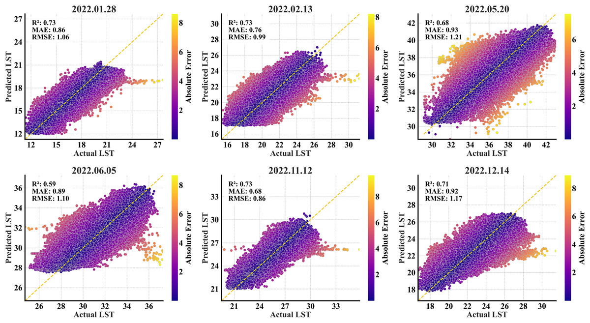
Figure 10: XGBoost scatterplots of the predicted refined LST (y-axis) vs. actual Landsat 9 LST (x-axis) data at 90 m for the secondary region; the yellow dashed diagonal line represents the 1:1 ideal line.
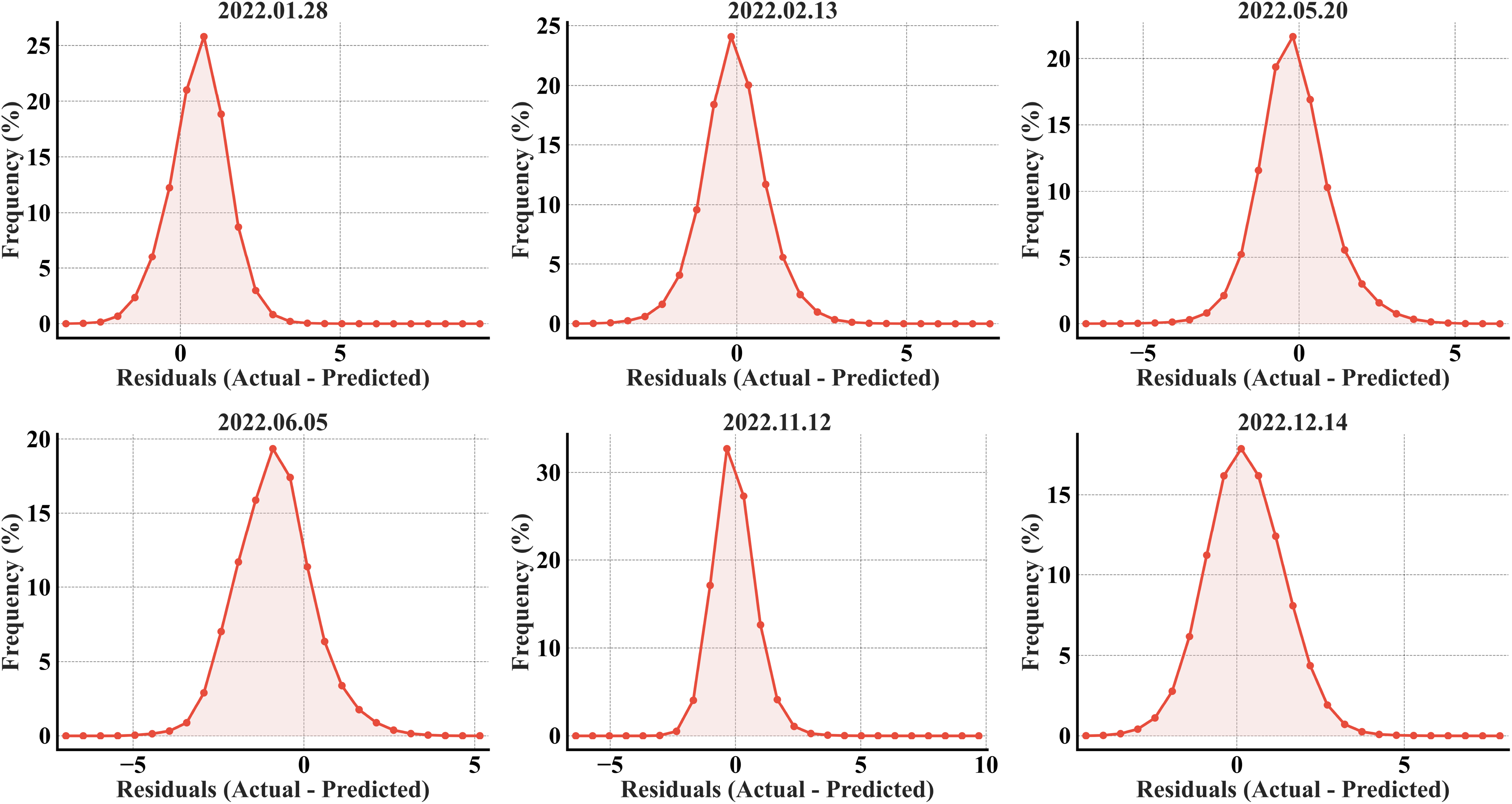
As illustrated in Fig. 11, the residual distribution for the XGBoost model in the secondary region is broadly comparable to the RF model. However, a key distinction appears in the November and December plots, where the RF model exhibits elongated right tails. These tails signify large-magnitude errors that are notably absent in the XGBoost results. Despite this, the RF model achieved a lower overall RMSE because of its higher volume of extremely accurate (near-zero error) predictions, effectively outweighing the statistical penalty from the infrequent outliers.
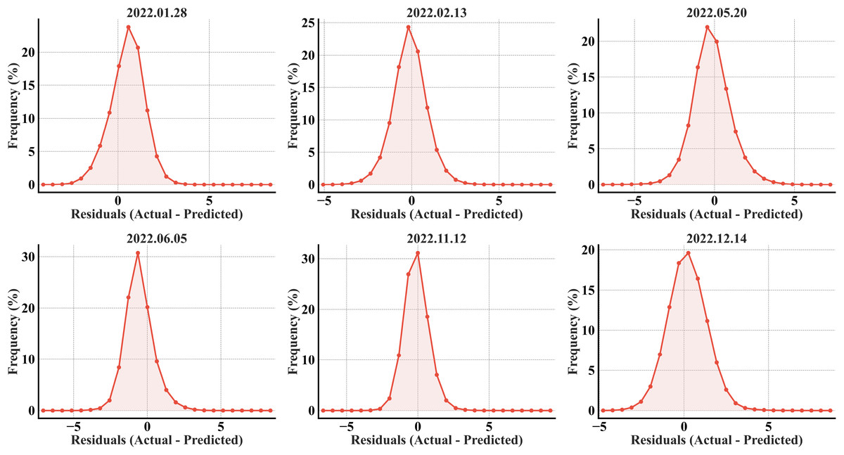
Figure 11: XGBoost error histograms from the predicted refined LST across all acquisition dates for the secondary region; the x-axis represents the prediction error in °C, and the y-axis represents the percentage of total pixels.
In contrast, the CatBoost model consistently straggled behind the RF model across all the evaluated months and metrics on the primary region’s test set (Table 8). CatBoost produced higher mean absolute error (MAE) and RMSE values and lower R2 scores than RF in all the months. In May, CatBoost’s RMSE and R2 were 0.75 and 0.88 respectively, both notably worse than the RF’s RMSE of 0.65 and R2 of 0.91. This pattern of weak performance was consistent, as observed in December, where CatBoost’s RMSE and R2 were 0.79 and 0.71 respectively, compared to the RF’s more accurate RMSE (0.72) and R2 (0.76). In the secondary region, the CatBoost model managed to match or even slightly outperform RF in a few months, e.g., in February, when its RMSE was 0.95 (Table 9) compared to RF’s 0.96 (Table 5) and November, when its RMSE was 0.84 compared to RF’s 0.85. But it experienced a pronounced failure in June. In this month, its R2 declined to just 0.32 (Fig. 12), whereas the RF model maintained an R2 of 0.65 (Fig. 6). This extreme inconsistency makes CatBoost unstable and therefore, inapposite for downscaling as a generalized model based on this study.

Figure 12: CatBoost scatterplots of the predicted refined LST (y-axis) vs. actual Landsat 9 LST (x-axis) data at 90 m for the secondary region; the yellow dashed diagonal line represents the 1:1 ideal line.
The CatBoost residuals plots (Fig. 13) exhibit close similarity with XGBoost in the months of January and May. Wider distributions can be observed in CatBoost in the months of June and December compared to XGBoost. Though inconsiderable in frequency, residuals of magnitude greater than 5 °C and extending up to 10 °C can be observed in the month of November in CatBoost. All the CatBoost residual plots show wider distributions for all the months, contrasting with the RF plots that depict strong concentration of residuals within ±2 °C.
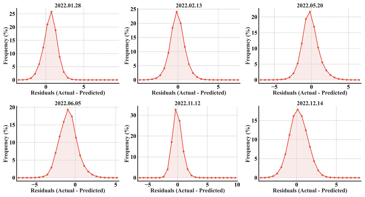
Figure 13: CatBoost error histograms from the predicted refined LST across all acquisition dates for the secondary region; the x-axis represents the prediction error in °C, and the y-axis represents the percentage of total pixels.
Discussion
The accurate downscaling of LST data is essential for applications in agriculture, forestry, and climate change studies. For this, the primary aim of the present study is to downscale MODIS LST from 1,000 m to 90 m in similar geo-environmental conditions using an RF regression model. In this regard, the exact retrieval dates of Landsat 9 and MODIS LST were considered for validation across different months. The study identifies key predictors affecting LST downscaling and assesses the model’s performance in the primary and secondary regions.
The feature importance analysis revealed that MODIS LST, SWIR1, and DEM consistently ranked as the most influential factors across all the temporal points. In contrast, the SAVI, blue band, and NIR band ranked as the lesser important variables (Fig. 3). In the study by Njuki, Mannaerts & Su (2020), the vegetation indices (NDVI, enhanced vegetation index (EVI), SAVI, and fractional vegetation cover (FVC)) and DEM were found to be the most important variables, while the reflectance bands had little role in spatial downscaling of LST. The addition of MODIS LST as an independent variable in the present study improved the model performance significantly, while the reflectance bands (except SWIR1) were less influential in both studies. This pattern aligns with broader applications of RF regression in LST downscaling, as shown by Hutengs & Vohland (2016), improving accuracy by up to 19% over the TsHARP method, and (Ebrahimy et al., 2021), adapting the same approach to various Köppen climate zones. These studies underscore that including terrain and vegetation-related variables (and, more generally, relevant environmental predictors) is crucial for accurate temperature predictions. The feature importance pattern underlines the shifting of environmental factors with transitions to different months.
The overall downscaling results validate the effectiveness of the RF regression model in both primary and secondary regions. A notable finding emerged in the cross-regional validation across different months, wherein in November and December, the model demonstrated more consistent performance across both regions than in May and June. The notably narrower temperature ranges in November and December than in May and June, highlighting seasonal variations in climate patterns, can be attributed to the consistent performance. The secondary region’s lower R2 and higher RMSE values stemmed from the region’s distinct climatic, topographic, and land-use conditions. In January and December, higher variability in the actual temperatures compared to the predictions highlighted the model’s limited capability in capturing regional heterogeneity. The spatially explicit RMSE patterns point to the potential benefits of localized model calibration. The overall transferability results make the RF model suitable for LST applications in similar environments.
The comparative analysis of RF with XGBoost and CatBoost was crucial for acknowledging its predictive capability within the broader landscape of machine learning models for LST downscaling. These models were specifically chosen in this study to balance the trade-off between the simpler machine learning approaches that often lack in simulating complex relationships in the data and deep learning frameworks that require a lot of training data and computation power. While all the models, notably the RF and XGBoost, performed comparably in the primary region’s test set, their limitations became evident in the new setting, with a marked decline in performance for XGBoost, and, more severely, for CatBoost specifically in the May and June months. The degraded performance can be attributed to the elevation differences between the primary and secondary regions. The distribution and characteristics of land cover types across varying elevations affect vegetation indices like SAVI and their relationship with LST (Wang et al., 2025; Song et al., 2025). Further, May and June are critical periods for vegetation growth and phenological changes, e.g., green-up, peak biomass in many regions. The relationship between LST and vegetation indices can be highly dynamic and vary significantly with seasonal changes (Sun & Kafatos, 2007; Karnieli et al., 2010; Ganguly et al., 2010; Gao & Zhang, 2021). A notable spatial disparity in temperature ranges was observed during the May and June months. While the primary region exhibited temperature ranges of 13.92 °C and 12.58 °C for May and June, respectively, the secondary region recorded significantly wider ranges of 16.90 °C and 14.70 °C for the same months, marking them as the broadest temperature variations across all assessed periods in that region. This forces the models to extrapolate beyond the variability they learned during training. The November and December months generally have lower solar radiation, cooler temperatures, and more stable atmospheric conditions with vegetation undergoing steady changes resulting more stable LST-feature relationships. Consequently, this environmental consistency enables the models to better generalize the learned relationships and produce better downscaling results.
The downscaling results indicate that month-specific calibration is essential for capturing seasonal variations in environmental and atmospheric conditions, thereby improving model performance. Additionally, regional adaptation is particularly crucial for months like May and June, where significant variations in climate, topography, and land-use patterns necessitate localized adjustments. Incorporating additional environmental parameters during model training could further enhance accuracy and robustness. These insights underscore the importance of spatiotemporal customization in modeling and highlight the potential benefits of a more comprehensive approach with a broader range of environmental factors. The methodology and results of this research will be helpful in sustainable agricultural practices and forest management in regions with similar geo-environmental conditions.
Conclusions
This study demonstrates the efficacy of RF regression in downscaling MODIS LST, emphasizing the importance of integrating multiple variables to achieve high predictive accuracy. The model’s performance was validated in the primary region and successfully applied to a spatially distinct secondary region, exhibiting its transferability. The RF model was also tested against XGBoost and CatBoost for contextual integrity and robustness.
Though the present work produced highly accurate downscaled images of LST in both primary and secondary regions using the RF regression model, it has limitations that suggest several avenues for future research. These include: employing hybrid machine learning models and advanced deep learning architectures to enhance spatial downscaling of LST; integrating more diverse environmental datasets into the existing models, such as soil moisture, atmospheric parameters, etc., to improve predictive accuracy; assessing the model’s performance across different geographic regions with unique climatic and land cover conditions to enhance generalizability; developing an automated framework for real-time LST downscaling to support climate monitoring, agriculture, and UHI studies; and validating the model with uncrewed aerial vehicle (UAV) and field observation datasets. These future advancements will make machine learning and deep learning-based downscaling a more robust and scalable solution for high-resolution thermal mapping.