Empirical copula-based data augmentation for mixed-type datasets: a robust approach for synthetic data generation
- Published
- Accepted
- Received
- Academic Editor
- Shibiao Wan
- Subject Areas
- Artificial Intelligence, Data Mining and Machine Learning
- Keywords
- Data augmentation, Copula, Machine learning, Generative augmentation technique
- Copyright
- © 2025 Ben Hassine and Mili
- Licence
- This is an open access article distributed under the terms of the Creative Commons Attribution License, which permits unrestricted use, distribution, reproduction and adaptation in any medium and for any purpose provided that it is properly attributed. For attribution, the original author(s), title, publication source (PeerJ Computer Science) and either DOI or URL of the article must be cited.
- Cite this article
- 2025. Empirical copula-based data augmentation for mixed-type datasets: a robust approach for synthetic data generation. PeerJ Computer Science 11:e3228 https://doi.org/10.7717/peerj-cs.3228
Abstract
Data augmentation is a critical technique for enhancing model performance in scenarios with limited, sparse, or imbalanced datasets. While existing methods often focus on homogeneous data types (e.g., continuous-only or categorical-only), real-world datasets frequently contain mixed data types (continuous, integer, and categorical), posing significant challenges for synthetic data generation. This article introduces a novel empirical copula-based framework for generating synthetic data that preserves both marginal and joint probability distributions and dependencies of mixed-type features. Our method addresses missing values, handles heterogeneous data through type-specific transformations, and introduces controlled noise to enhance diversity while maintaining statistical fidelity. We demonstrate the efficacy of this approach using synthetic and experimental benchmark datasets such as the Census Income and the Wisconsin Diagnostic Breast Cancer (WDBC) dataset, demonstrating its ability to generate realistic synthetic samples that retain the statistical properties of the original data. The proposed method is implemented in an open-source Python class, ensuring reproducibility and scalability.
Introduction
The growing demand for robust machine learning models has highlighted the importance of data augmentation, particularly in domains where data scarcity or privacy constraints limit access to large datasets (Bayer et al., 2023; Cubuk et al., 2019; Dao et al., 2019; Feng et al., 2021; Inan, Hossain & Uddin, 2023; Mumuni, Mumuni & Gerrar, 2024). Traditional augmentation techniques, such as Synthetic Minority Over-sampling Technique (SMOTE) for tabular data (Kotelnikov et al., 2023; Chawla et al., 2002), generative adversarial networks (GANs) (Goodfellow et al., 2014; Xu et al., 2019; Engelmann & Lessmann, 2020; Park et al., 2018; Yang et al., 2024) for image data, or Synthetic Data Vault with Gaussian Copula (SDV-G) (Patki, Wedge & Veeramachaneni, 2016) or variational autoencoders (VAEs) (Chadebec & Allassonnière, 2021) for generative modeling often struggle with mixed-type datasets (Jiang et al., 2021) containing continuous, integer, and categorical variables. These methods typically fail to preserve complex dependencies between heterogeneous features, leading to synthetic data that poorly reflect real-world probability distributions (Endres, Mannarapotta Venugopal & Tran, 2022; Goyal & Mahmoud, 2024).
Copula theory, which models multivariate probability distributions by separating marginal probability distributions from their dependence structure, offers a promising solution (Restrepo et al., 2023; Kamthe, Assefa & Deisenroth, 2021). However, existing copula-based approaches are largely parametric (Benali et al., 2021) and require assumptions about the underlying distribution (Simon & Tibshirani, 2014), limiting their applicability to empirical datasets. This article bridges this gap by proposing a non-parametric empirical copula framework that (1) handles missing values through imputation or deletion, (2) transforms mixed-type features into uniform margins while preserving ordinality and categorical relationships, (3) generates synthetic data by resampling from the empirical copula and inverse-transforming to the original space, and (4) introduces configurable noise to enhance diversity without distorting statistical properties.
The proposed empirical copula-based method offers a significant advantage over SDV-G, which assumes a Gaussian copula for data generation. The Gaussian copula inherently imposes a normal dependence structure, limiting its ability to model complex, non-linear relationships like asymmetric or tail-dependent relationships present in real-world datasets. In contrast, our empirical copula approach is fully data-driven, capturing the true joint probability distribution without restrictive parametric assumptions. Additionally, SDV-G struggles with heterogeneous data types, requiring manual preprocessing to encode categorical and ordinal variables, whereas our method integrates type-specific transformations to seamlessly handle mixed data. Furthermore, the empirical copula technique preserves the marginal probability distributions of the features more accurately, ensuring that synthetic samples maintain statistical fidelity to the original dataset (Houssou et al., 2022). By avoiding rigid Gaussian constraints, our method generates more realistic and diverse synthetic data, making it more suitable for tasks requiring high-fidelity augmentation.
This article is organized as follows. In ‘Dependence Modeling Challenges’, we introduce copula theory, discussing its foundational concepts and the definition of the empirical copula function. This section lays the groundwork for understanding the statistical properties of copulas, which are pivotal to our proposed data augmentation methodology. In ‘Theoretical Framework of the Data Generator’, we present a detailed exploration of our methodology. This section not only outlines the technical framework of the empirical copula-based approach but also delves into the key challenges encountered in dealing with mixed data types, such as continuous, integer, and categorical features. We describe the underlying strategies implemented to address these challenges and provide deep insights into how our method ensures both statistical fidelity and enhanced data diversity. In ‘Assessment and Results’, we present a comprehensive evaluation of our method. We conduct a series of simulations using benchmark datasets, demonstrating the efficacy of our approach in generating realistic synthetic data while preserving the original probability distribution and dependencies of the data in realistic time. We analyze and interpret the results to validate the strengths and limitations of our method. Finally, in ‘Broader Implications, Challenges, and Future Directions’, we discuss the broader implications of our work. We highlight the challenges encountered during the study, outline potential avenues for future research, and propose directions for enhancing the scalability and versatility of our approach.
Dependence modeling challenges
Copula theory offers a powerful statistical framework to model the dependence structure among random variables while decoupling this structure from the marginal probability distributions. This capability is particularly important when working with datasets containing mixed data types—continuous, integer, and categorical—where standard techniques often fall short. In this section, we introduce the core concepts of copula theory and define the empirical copula function. We also describe how our methodology addresses the challenges posed by mixed data types during the computation of the empirical copula.
At its essence, a copula is a multivariate cumulative probability distribution function that “couples” univariate marginal probability distribution functions to form a joint probability distribution. This is formalized by Sklar’s Theorem, which states that any multivariate joint probability distribution function, H(x1, x2,…, xd), can be expressed as
where represents the cumulative probability distribution function (CPDF) of the i-th variable, and C is the copula capturing the dependency among these variables. Importantly, by transforming each marginal probability distribution into a uniform probability distribution on the interval [0,1], copulas isolate the dependency structure, thereby providing a flexible means of modeling both linear and non-linear relationships.
In practice, the theoretical copula is approximated using the empirical copula function, Cn, a non-parametric estimator derived directly from observed data. Given a sample of n observations , Cn is defined as
where is the indicator function and Fi is the empirical CPDFs of the respective variables. This approach maps observed data to the unit hypercube, facilitating the estimation of the joint dependence structure.
A central challenge in employing the empirical copula framework is the proper handling of mixed data types. Since copulas naturally operate on continuous variables, special strategies must be adopted for integer and categorical data as follows. For continuous data, the conversion to uniform margins is achieved by ranking the data and then normalizing these ranks. This transformation is straightforward and retains the original data’s structure. For integer data, although they are discrete, they often represent measurements that could be approximated as continuous with slight adjustments. To address this problem, we introduce a controlled amount of noise—commonly referred to as “jittering”—to the integer data before applying the rank transformation. This mitigates the issues arising from their discrete nature while preserving the inherent probability distribution and relationships. As for categorical data, they do not possess a natural ordering, which complicates their transformation. To incorporate them into the copula framework, we transform categorical values into a probabilistic representation. This is achieved by assigning each category its empirical cumulative probability, thus mapping categorical data onto the uniform [0,1] scale. This approach allows us to capture dependencies between categorical variables and those of other types without losing their distinct, non-numeric characteristics.
By implementing these tailored transformations, the empirical copula function can effectively capture the complex dependence structures present in mixed-type datasets. This is essential for our data augmentation methodology, which relies on accurately preserving both marginal properties and inter-variable dependencies in the synthetic data. The application of the empirical copula function in our methodology enables the generation of synthetic data that mirrors the original dataset’s statistical properties. By carefully addressing the nuances of continuous, integer, and categorical data through specific transformation techniques, our approach ensures that the synthesized data accurately retains the inherent dependency structure. This is particularly critical in scenarios where traditional augmentation methods fail to capture the diversity and complexity (Yang, Shen & Zhao, 2024) of mixed data types.
Theoretical framework of the data generator
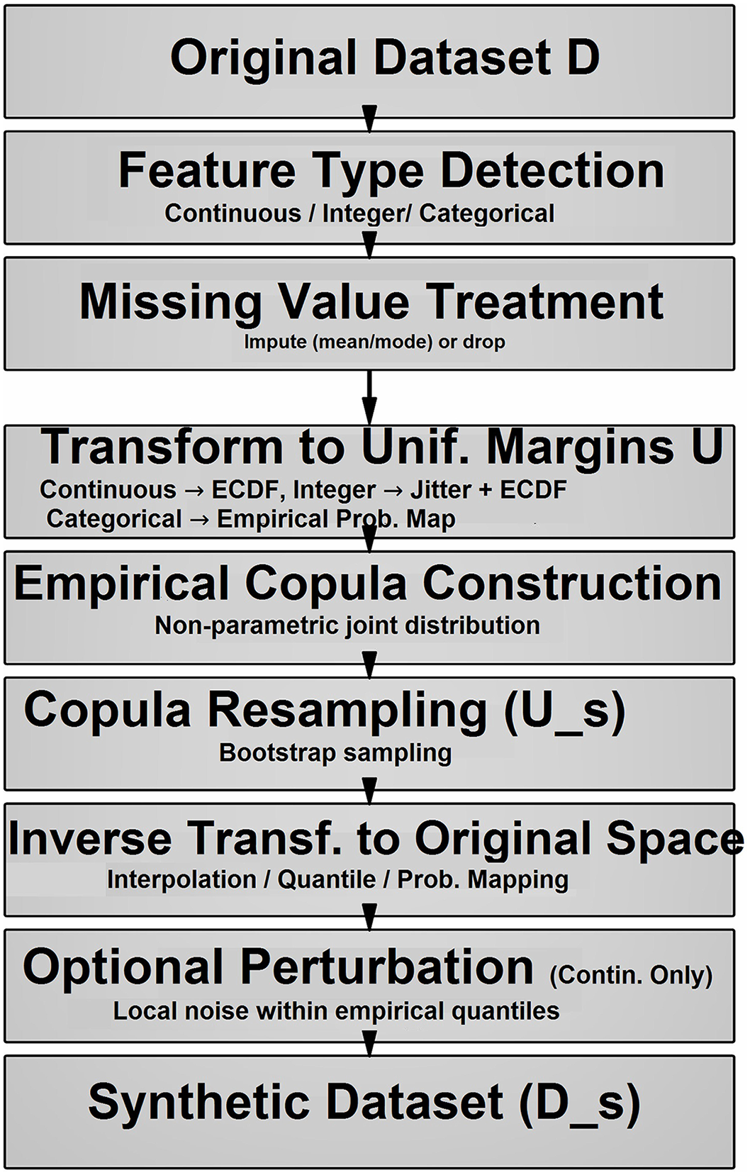
In this section, we present the theoretical foundations and algorithmic constructs of the Empirical Copula Generator (ECG), a method designed to synthesize data that preserve the distributional and dependence properties of an input dataset with mixed types—continuous, integer, and categorical. We address missing data treatment, mixed data handling, perturbation strategies, empirical copula computation, inverse transformations, and augmented data generation. Each subsection pairs a detailed theoretical discussion with a mathematically notated algorithm corresponding to specific functions in the implementation. Figure 1 summarizes the workflow of the proposed empirical copula-based data generator. It outlines the main phases: (1) missing data handling, (2) mixed-type transformation, (3) copula fitting and resampling, and (4) inverse transformation to produce augmented data.
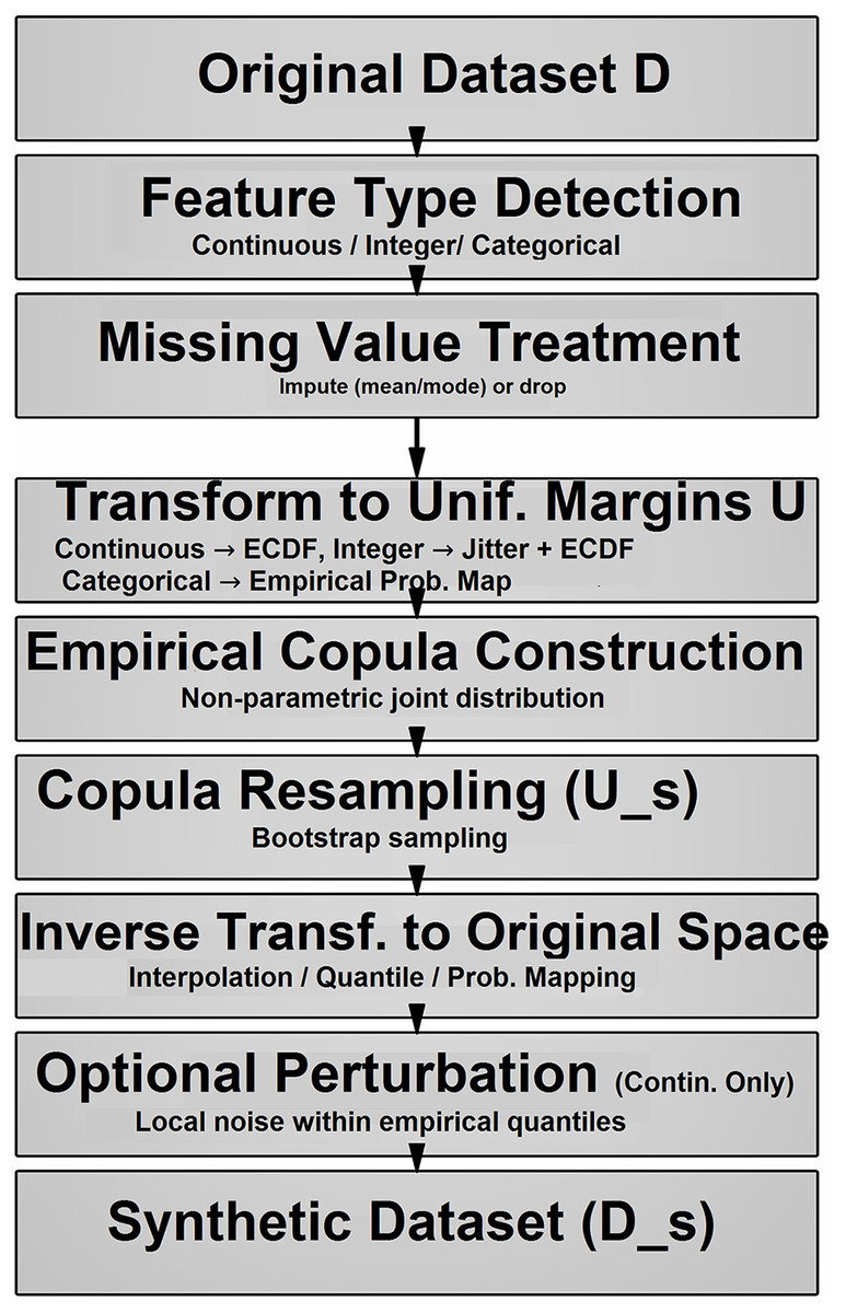
Figure 1: The workflow of proposed empirical copula-based data generator.
Treatment of missing data
Real-world datasets often contain missing values, necessitating preprocessing to enable subsequent modeling. The ECG offers two strategies: imputation, which fills missing entries with statistically derived substitutes, and exclusion, which removes incomplete observations.
Imputation: For numerical variables (continuous or integer), missing values are replaced with the column mean or any convenient function), leveraging central tendency to maintain distributional coherence. For categorical variables, the mode, the most frequent category is used, preserving discrete structure. This maximizes data retention, suitable for moderate deficiency.
Exclusion: Rows with any missing values are discarded, ensuring a complete dataset at the cost of reduced sample size, this is ideal when data incompleteness is minimal.
The algorithm takes as input a dataset D ∈ and a strategy S ∈ {impute, drop}, and outputs a processed dataset D′. Initially, D′ is set equal to D. If the strategy S is “impute”, the algorithm iterates over each column j = 1,…,m. For each numerical columns D[:,j], it computes the mean of the non-missing values and replaces missing entries in D′[:,j] with . For categorical columns, it computes the mode and fills in missing values with . If the strategy is “drop”, the algorithm removes all rows D[i,:] that contain missing values in any column j, resulting in a cleaned dataset D′. Finally, it returns D′ as result.
Handling mixed data types
The heterogeneity of data types—continuous, integer, and categorical—needs a nuanced approach to modeling and transformation. The ECG adeptly categorizes and processes each variable according to its intrinsic properties, a foundational step that enables the separation of marginal probability distributions from their dependence structure, a hallmark of copula theory.
Detection type: The method begins by classifying each variable. Continuous variables are identified as those capable of assuming any real value within a range, typically represented numerically with floating-point precision. Integer variables, while numeric, are discrete and confined to whole numbers, often requiring special handling to approximate continuity. Categorical variables, encompassing nominal or ordinal data such as labels or categories, resist numerical conversion and are treated as discrete variables. This classification is pivotal, as it dictates the subsequent transformation strategy, ensuring that the probability distribution characteristics of each variable are appropriately captured.
Transformation to uniform margins: Copula theory states that any multivariate probability distribution can be decomposed into its marginal probability distributions and a copula that encapsulates their dependence. To isolate this dependence, each variable is transformed to a uniform distribution over [0,1], a process that standardizes the margins while preserving inter-variable relationships. For continuous variables, this transformation employs the empirical cumulative probability distribution function (ECPDF), where the rank of each observation within the sorted data is normalized by the sample size. This rank-based approach yields a pseudo-uniform probability distribution, reflecting the shape of the ECPDF without parametric assumptions. Integer variables, inherently discrete, undergo a preliminary jittering process, where small random perturbations are added to break ties and simulate a continuous probability distribution, followed by the same rank-based transformation. Categorical variables, lacking a natural ordering, are mapped to the unit interval based on their cumulative frequencies: each category is assigned a uniform value proportional to its position in the cumulative probability distribution, effectively discretizing the [0,1] range according to category prevalence.
| Input: Dataset D ∈ , strategy S ∈ {impute, drop} |
| Output: Processed dataset D′ |
| D’=D |
| If S=“impute”: |
| For each column j = 1,…,m: |
| If D[:,j] is numerical : |
| Compute = mean(D) |
| Set D’[i:,j] = |
| Else (categorical): |
| Compute mode = mode (D) over non missing values |
| Set D’[i:,j] = |
| Else (S=“drop”) |
| Set D’={D[I,:] where D[i:,j] is not missing} |
| Return D’ |
The algorithm takes as input a dataset D ∈ and outputs a list T = [t1,…, tm], where each tj indicates the data type of column j. For each column j = 1,…,m, it attempts to convert the values D[:,j] to float type, stored in F[:,j]. If the conversion is successful, it further tries to convert them to integers I[:,j]. If all values in F[:,j] equal those in I[:,j], the column is classified as ‘integer’; otherwise, it is ‘continuous’. If the initial float conversion fails, the column is labeled as ‘categorical’. The algorithm returns the list T, indicating the detected type for each column.
| Input: Dataset D ∈ |
| Output: Type list T = [t1,…tm] |
| For each column j = 1,..,m: |
| Try converting D[:,j] to floats F[i,j] |
| If successful: |
| Convert D[:,j] to integers I[i,j] |
| If F[:,j] = I[:,j]: |
| tj=‘integer’ |
| else: |
| tj= ‘continuous’ |
| else: |
| tj=“categorical” |
| Return T |
The algorithm transforms a column C ∈ into a uniform distribution on [0, 1], based on its type ∈ {continuous, integer, categorical}, with optional noise scale . If t = “continuous”, it computes the rank R[i] of each value as the proportion of entries less than or equal to C[i], then sets U[i] = (R[i]−1)/n. If t = “integer” it adds small random noise to each value (jittering), forming C′[i] = C[i] + , then computes ranks R′[i] and uniform values as before. If t = “categorical”, it first determines the set of unique values V = {v1,…,vk}, then estimates their relative frequencies N[vl], and computes the cumulative probability P(vl). Each value C[i] is then mapped to its corresponding cumulative probability U[i] = P(vl). The output is the transformed column U ∈ , uniformly distributed.
Perturbing continuous data
To ensure that generated data introduces novelty rather than merely replicating the original observations, the method incorporates a controlled perturbation mechanism for continuous variables. This step is theoretically motivated by the need to balance fidelity to the original probability distribution with the generation of plausible variations, a critical aspect of data augmentation.
Perturbation mechanism: For each uniform value derived from a continuous variable, the method identifies its position within the sorted original data. Adjacent values—termed neighbors—define the local context, establishing bounds within which perturbation can occur without disrupting the order of the data. The maximum allowable noise is calculated as the minimum distance to these neighbors, ensuring that the perturbed value remains consistent with its rank. A small random noise, scaled by a predefined factor, is then added within this range, and the perturbed uniform value is mapped back to the original scale via an inverse transformation. This process introduces subtle variations, mimicking natural variability while preserving the distributional properties and dependence structure.
The algorithm perturbs a continuous column X ∈ , using a reference sorted column C, its corresponding uniform transformation U ∈ , and a noise scale ε, to generate perturbed data X′ ∈ . It begins by sorting C to obtain the ordered list S = [s1,…,sn]. For each value v = X[i], it finds the interval [sk, sk+1] that contains v, and sets the bounding values v1 = smax(1,k-1), and v2 = smin(k+1,n). The maximum noise magnitude η is the smaller of the distance from v to either bound, or 0.01 if both bounds are equal. Then, a uniform random noise z∼Unif (−1, 1) is scaled by η⋅ε and added to v to produce U′[i], which is clipped to [0,1]. Finally, X′[i] is obtained by applying the inverse CDF of C to U′[i], and the perturbed vector X′ is returned.
| Input: Column C ∈ , type t, noise scale ε |
| Output: uniform column U ∈ |
| If t=”continuous”: |
| Compute ranks R[i]= |
| U[i] = (R[i]-1)/(n-1) |
| Else if t=”integer”: |
| Jitter: |
| Compute ranks R’[i]= |
| U[i] = (R’[i]-1)/(n-1) |
| Else: |
| Compute unique values V = {v1,…vk} |
| Counts N[vl] = |
| Compute cumulative prob as: |
| Set U[i] = where |
| Return U |
Computing the empirical copula
The empirical copula serves as the linchpin of this methodology, providing a non-parametric estimate of the dependence structure among variables. Grounded in copula theory, this construct captures the joint behavior of the transformed uniform margins, enabling the generation of new data that respects observed interdependencies.
Construction process: After transforming all variables to uniform margins, the empirical copula is implicitly defined by the joint probability distribution of these uniform variables. Rather than fitting a parametric copula model, the method retains the empirical joint probability distribution as observed in the data, leveraging the ranks and their multivariate configuration. This non-parametric approach eschews assumptions about the functional form of the copula, relying instead on the inherent structure of the data.
Sampling mechanism: To generate new samples, the method employs resampling with replacement from the uniform dataset. Each sampled row represents a realization of the empirical copula, preserving the observed dependence through the co-occurrence of uniform values across variables. This resampling mirrors the bootstrap technique, adapted here to synthesize new multivariate observations rather than estimate statistical properties.
| Input: Column C ∈ , U ∈ , X ∈ |
| Output: Perturbed data X′ ∈ |
| Sort C to get S = [s1,..sn] |
| For each i = 1,..n: |
| Set v = X[i], find k such that sk≤ v ≤ sk+1 |
| Compute v1 = smax(1,k-1), and v2 = smin(k+1,n) (bounds of v) |
| Compute max noise as follows: |
| If v1 ≠ v2: |
| Else: |
| Perturb U’[i] = v + .z, where z ~Unif (−1, 1) |
| Clip U’ ∈ |
| X′ [i] = inverse CDF (U’[i]) |
| Return X′[i] |
Algorithm 5 takes a dataset D ∈ with a noise scale ε, and transforms it into a matrix U ∈ with uniform margins, suitable for copula modeling. First, it applies the Handling Missing Value procedure to produce a clean dataset D′. Then, it uses Detecting Column Names to infer the type T = [t1,…,tm] for each column in D′. For every column j = 1,…, it applies Transforming to Uniform Margins to the column D′[:,j], using its type T[j] and noise scale ε, resulting in a uniform column U[:,j]. The final output U is a uniformly transformed version of the data, preserving the dependence structure across features.
| Input: Dataset D ∈ , n |
| Output: U ∈ |
| D’= Handling Missing Value (D) |
| T = Detecting column names (D’) |
| For each j = 1,..m |
| U [:, j] = Transforming to uniform margins (D’[:,j],T[j], |
| Return U |
Algorithm 6 generates new samples Us ∈ from a previously fitted copula represented by U ∈ , using a specified sample size ns. It begins by drawing ns random indices I = [i1,…,ins], each sampled independently with replacement from the set {1,…,n}, following a uniform distribution. For each k = 1,…,ns, it sets the new sample row Us[k,:] = U[ik,:]. The resulting matrix uspreserves the empirical dependency structure from U, making it a valid synthetic dataset on the uniform scale.
| Input: U ∈ , sample size ns |
| Output: Us ∈ |
| Draw indices I= [i1,…, ins] where ik ~Unif[1,n] with replacement |
| Set Us[k,:]=U[ik,:] for k:1,…ns |
| Return Us |
Inverse transformation via the empirical copula
Generating synthetic data in the original space requires reversing the uniform transformation, a process that reconstructs each variable’s marginal probability distribution from the sampled copula values.
Continuous variables: The inverse transformation for continuous variables approximates the quantile function (inverse CPDF) using the original data’s sorted values. Uniform samples are mapped to this empirical quantile function, often via interpolation to handle values between observed points. Post-mapping, the perturbation step described earlier introduces controlled noise, ensuring that the resulting values reflect both the original probability distribution and added variability.
Integer variables: For integers, the uniform samples are mapped to the nearest corresponding quantile in the original data, effectively rounding to the closest integer value. This preserves the discrete nature of the variable, aligning the synthetic data with its empirical probability distribution.
Categorical variables: Categorical variables are reconstructed by partitioning the [0,1] interval according to the original categories’ cumulative frequencies. Each uniform sample is assigned to the category whose cumulative probability range it falls within, replicating the discrete probability distribution observed in the input data.
This algorithm reverses the copula-based uniform transformation, mapping uniform samples Us ∈ back to their original data space using a reference column C ∈ and its type t ∈ {“continuous”, “integer”, “categorical”}. If t= “continuous”, it first sorts C to obtain S, defines a function f(u) that interpolates u ∈ [0,1] over S, then computes X = f(Us). The result is refined using the Perturbing Continuous Data algorithm to add realistic noise, producing Xs . If t = "integer", each Xs[i] is computed as the empirical quantile of C at Us[i]. For categorical data, it retrieves the unique values V and their cumulative probabilities P (as in Algorithm 3), and assigns Xs[i] = vl such that P(vl−1) < Us[i] ≤ P(vl). The final output is Xs, a column of data samples in the original scale.
Generating augmented data
The culmination of the ECG is the production of augmented data, achieved through an integrated workflow that synthesizes the preceding components. The process commences with preprocessing to handle missing data, followed by type detection and transformation to uniform margins, effectively fitting the empirical copula. New samples are then drawn from this copula via resampling, and each uniform sample is transformed back to the original space using the appropriate inverse method. The result is a synthetic dataset that mirrors the original’s marginal probability distributions and dependence structure, augmented with controlled variations for continuous variables.
This algorithm creates a synthetic dataset Ds ∈ from an original dataset D ∈ , using a sample size ns. First, it applies fitting the Copula to D to obtain the uniform representation U ∈ , which captures the dependence structure between features. Then, it uses sampling from the Copula to draw nsnew samples Us ∈ from U. For each column j = 1,…,m, the algorithm applies Inverse Transformation to Us[:,j], using the original column D[:,j] and its type T[j], to produce the synthetic column Ds[:,j]. The result is a fully synthetic dataset Ds, with the same feature structure and dependency patterns as the original data.
| Input: Us ∈ , C ∈ , type t |
| Output: transformed column Xs |
| If t=“continuous”: |
| S = sort(C) |
| Define f(u) = interp(u, [0, 1], S) |
| X = f(Us) |
| Xs = Perturbing_Continuous_Data(C, Us, X, |
| Else if t = “integer”: |
| Xs[i] = quantile(C, Us[i]) |
| Else : |
| Compute V and as in Algorithm 3 |
| Xs[i] = vl where (vl-1) < Us[i] ≤ (vl) |
| Return (Xs) |
| Input: Original dataset D ∈ , sample size ns |
| Output: Synthetic dataset Ds ∈ |
| U = Fitting_the_copula(D) |
| Us = Sampling_from_the _copula(U,ns) |
| For each j = 1,..m: |
| Ds[:,j] = Inverse_transformation(Us[:,j], D[:,j],T[j]) |
| Return Ds |
Advantages and theoretical considerations
The ECG offers several theoretical advantages:
Flexibility with mixed types: By tailoring transformations to each data type, it seamlessly accommodates heterogeneity, a common feature of real-world datasets.
Non-parametric nature: Its reliance on empirical probability distributions avoids restrictive parametric assumptions, enhancing applicability across diverse domains.
Dependence preservation: The resampling strategy ensures that multivariate relationships are retained, a critical factor in multivariate analysis.
Controlled variation: Perturbation introduces novelty without compromising statistical fidelity, enriching the synthetic output.
The ECG emerges as a robust theoretical framework for synthetic data generation, harmonizing copula theory with practical adaptations for mixed-type data. Its meticulous handling of missing values, type-specific transformations, perturbation mechanisms, and empirical copula construction culminates in a method that balances fidelity and innovation. This approach holds significant promise for advancing research in data science, offering a versatile tool for augmentation, privacy preservation, and beyond.
Assessment and results
In this section, we evaluate the efficacy of the ECG by systematically assessing the similarity between the original dataset and its synthetically augmented counterpart. Our assessment methodology leverages a suite of statistical tools designed to scrutinize both marginal distributions and joint dependence structures, ensuring a comprehensive validation of the method’s ability to replicate the statistical properties of the input data. We first elucidate the theoretical foundations of our evaluation framework, detailing the statistical tests and divergence measures employed to compare the original and augmented datasets. Subsequently, we present the empirical results of applying this framework to a representative dataset, highlighting the generator’s performance in preserving distributional fidelity and multivariate relationships.
Assessment methodology
To rigorously evaluate the synthetic data produced by the ECG, we developed a multifaceted assessment protocol that examines both univariate and multivariate properties. This approach ensures that the augmented data not only mirrors the individual feature distributions of the original dataset but also maintains the intricate interdependencies among variables. Below, we describe the theoretical constructs and statistical methodologies underpinning our evaluation, drawing from established techniques in probability distribution comparison and dependence analysis (Wang, Wang & Liu, 2025).
Identification of feature types
The initial step in our assessment involves classifying the features of the dataset into numerical (continuous or integer) and categorical types. This distinction is essential, as it dictates the appropriate statistical tools for subsequent comparisons. Numerical features, characterized by their capacity to assume a range of real or discrete integer values, are subjected to tests suited for continuous or near-continuous probability distributions. Categorical features, defined by discrete, non-numeric labels, require methods tailored to frequency-based probability distributions. This classification ensures that our evaluation respects the intrinsic properties of each variable, aligning the analysis with the mixed-type nature of the data processed by the ECG.
Comparison of marginal probability distributions
For each feature, we assess the similarity between its probability distribution in the original dataset and the augmented dataset using tailored statistical tests:
Numerical features: The Kolmogorov-Smirnov (KS) two-sample test is employed to compare the empirical cumulative probability distribution functions (ECPDFs) of the original and augmented data. The KS statistic, defined as where Forig(x) and Faug(x) are the ECPDFs of the original and augmented samples respectively, quantifies the maximum vertical distance between these probability distributions. The associated p-value tests the null hypothesis that both samples are drawn from the same underlying probability distribution. A low KS statistic and a high p-value (e.g., p > 0.05) indicates distributional similarity, suggesting that the generator effectively preserves the marginal probability distribution of the feature. To complement this statistical test, we visualize the probability distributions using kernel density estimates (KDE) overlaid on histograms. This graphical representation provides an intuitive assessment of how closely the augmented data mimics the original, revealing any discrepancies in shape, spread, or central tendency that might not be fully captured by the KS test alone.
Categorical features: To provide a holistic measure of similarity across all categorical features, we calculate the Jensen-Shannon (JS) divergence, a symmetric and bounded variant of the Kullback-Leibler divergence. For two probability distributions P and Q over a discrete space, the JS divergence is defined as where M = 1/2 (P+Q) is the mixture distribution and KL denotes the Kullback-Leibler divergence given by For categorical features, the empirical probability distributions are used directly, with appropriate normalization to account for all possible categories
Comparison of joint probability distributions
To evaluate the preservation of multivariate relationships, we employ two complementary approaches: correlation analysis and Jensen-Shannon (JS) divergence.
Correlation heatmaps: For numerical features, we compute the Pearson correlation coefficient matrix for both the original and augmented datasets. The correlation coefficient between two variables X and Y is given by where Cov(X,Y) is the covariance, and are the standard deviations. These matrices are visualized as heatmaps, allowing a direct comparison of the dependence structures. Close alignment between the heatmaps indicates that the ECG successfully retains the linear relationships among numerical variables, a key aspect of its copula-based resampling strategy.
Jensen-Shannon divergence: To provide a holistic measure of similarity across all features—numerical and categorical—we calculate the Jensen-Shannon (JS) divergence, the symmetric and bounded variant of the Kullback-Leibler divergence defined above.
This dual approach—correlation for numerical dependencies and JS divergence for overall distributional fidelity—offers a robust evaluation of the generator’s performance in capturing both local and global statistical properties.
Empirical results
Experiments on synthetic datasets
Synthetic datasets provide a controlled setting to assess the generator’s ability to replicate structured patterns, making them an ideal starting point for evaluation. We begin with experiments on the Star Shape dataset and the Multiple Forms dataset, conducted in sequence to test the method’s precision and robustness under varying noise conditions.
Star Shape dataset experiment
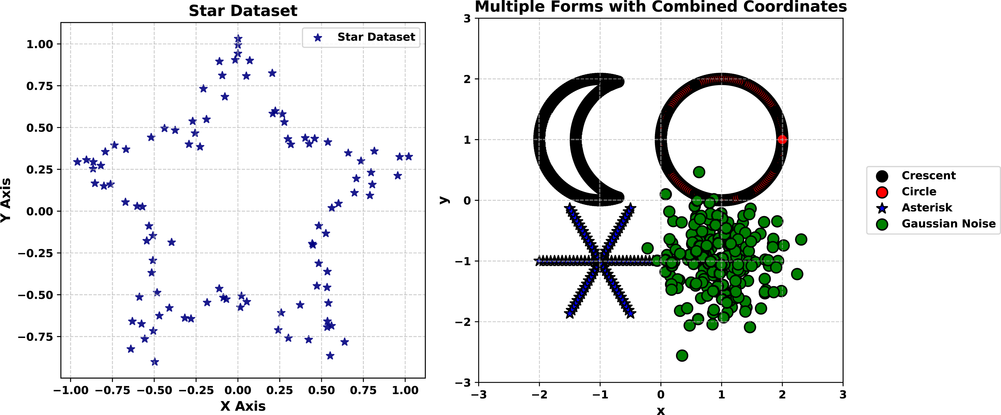
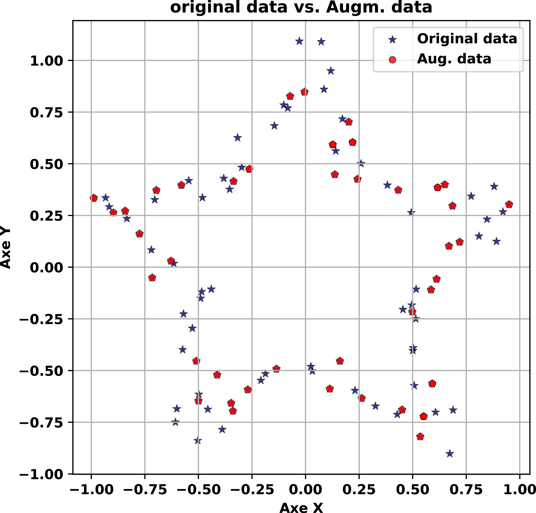
The first experiment focuses on the Star Shape dataset, comprising 100 points arranged in a five-armed star pattern with an initial noise perturbation of 0.05. This dataset tests the generator’s capacity to preserve a simple yet distinct geometric structure. The experiment progresses through three stages, each visualized in Figs. 2–4. The experiment begins with the original dataset, depicted in Fig. 2 as a scatter plot in blue. The five arms of the star are clearly defined, radiating symmetrically from the center despite the slight noise. This figure serves as the baseline, illustrating the target structure that the generator must replicate. The clarity of the star’s shape, even with minor perturbations, establishes a straightforward yet effective reference for evaluating synthetic outputs.
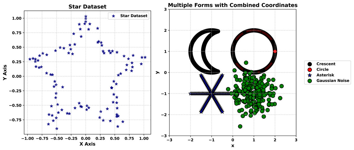
Figure 2: Star Shape and Multiple Forms datasets.
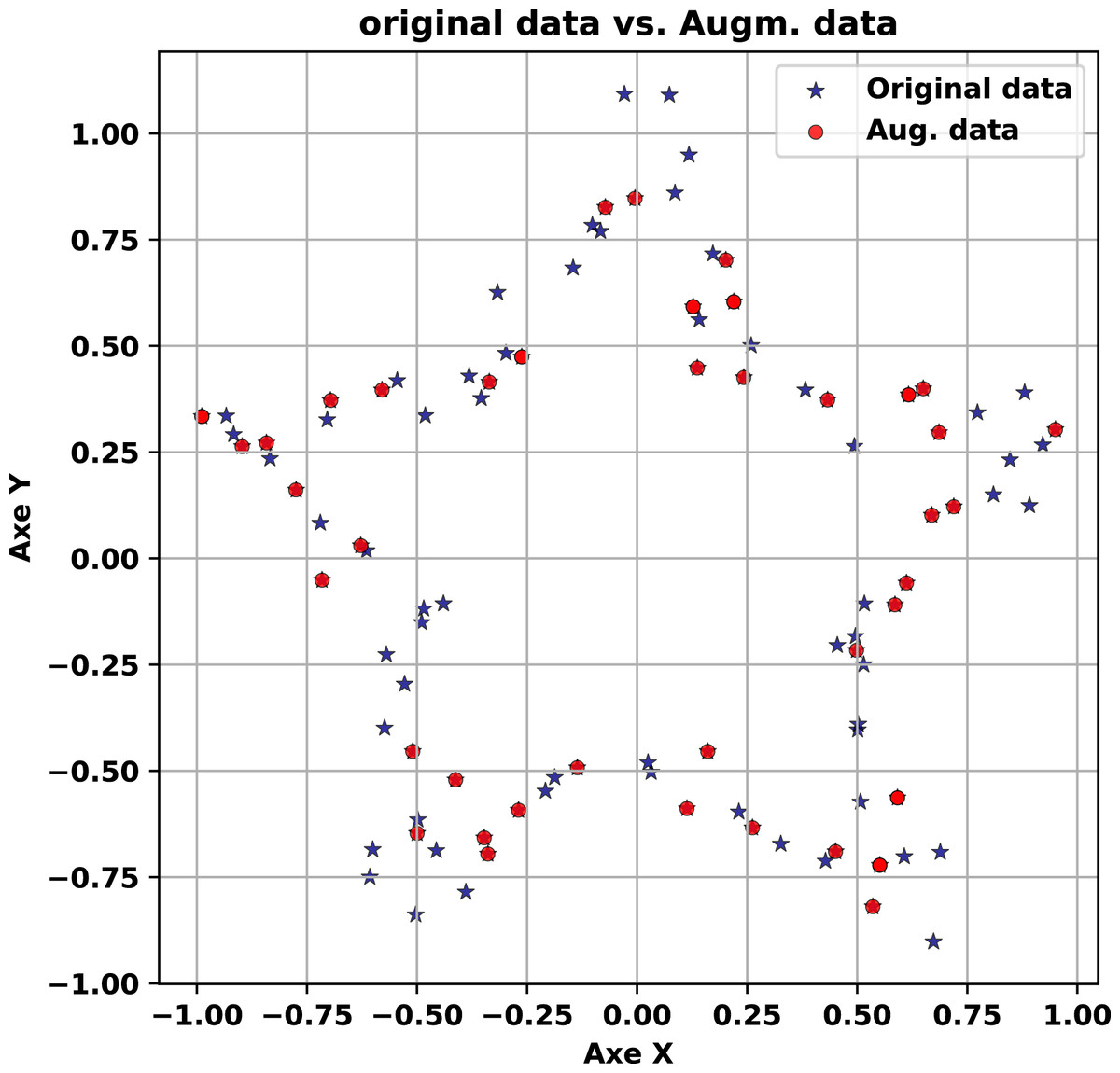
Figure 3: Empirical runtime scaling of data generator with respect to sample size and feature dimensionality.
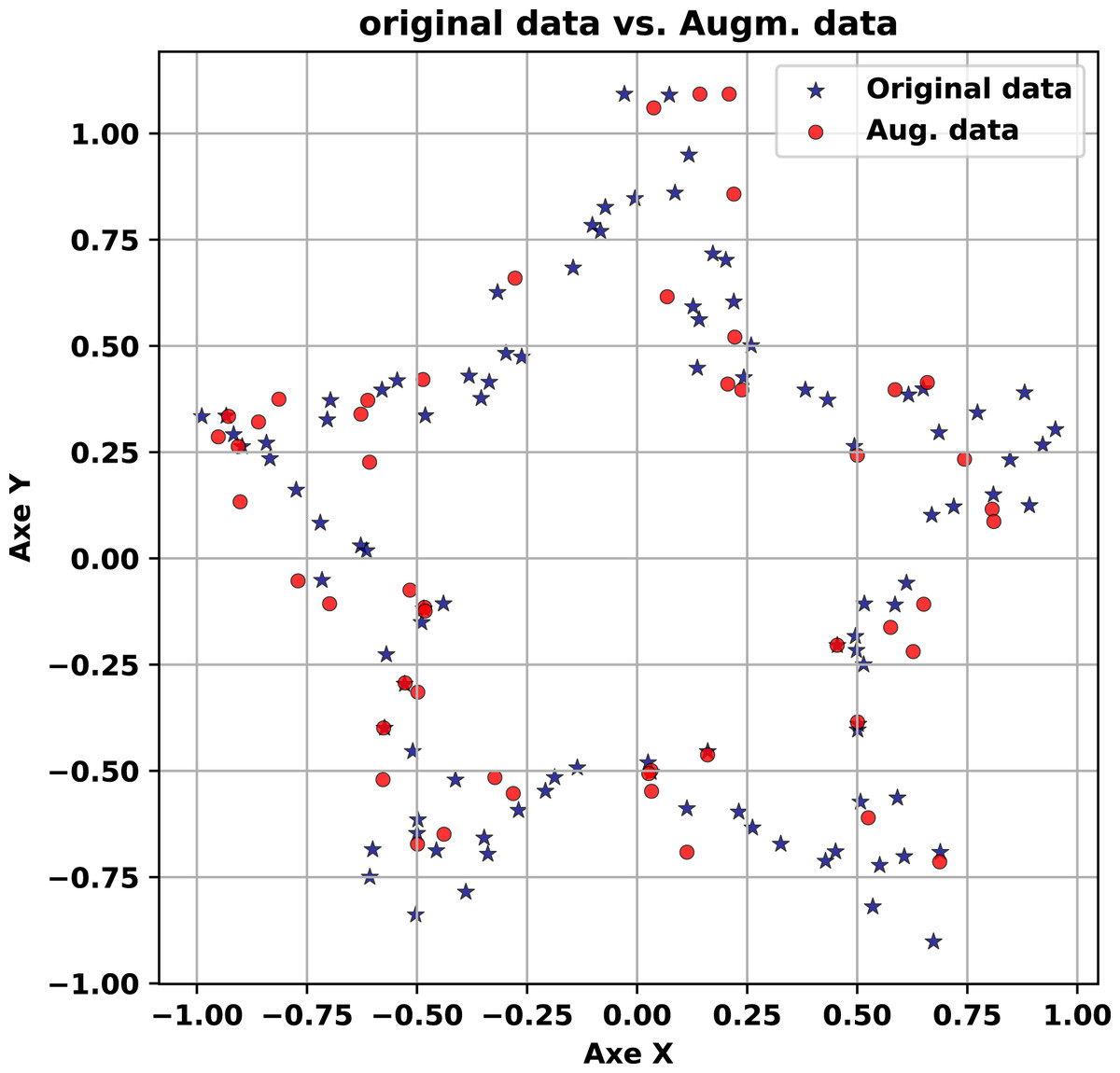
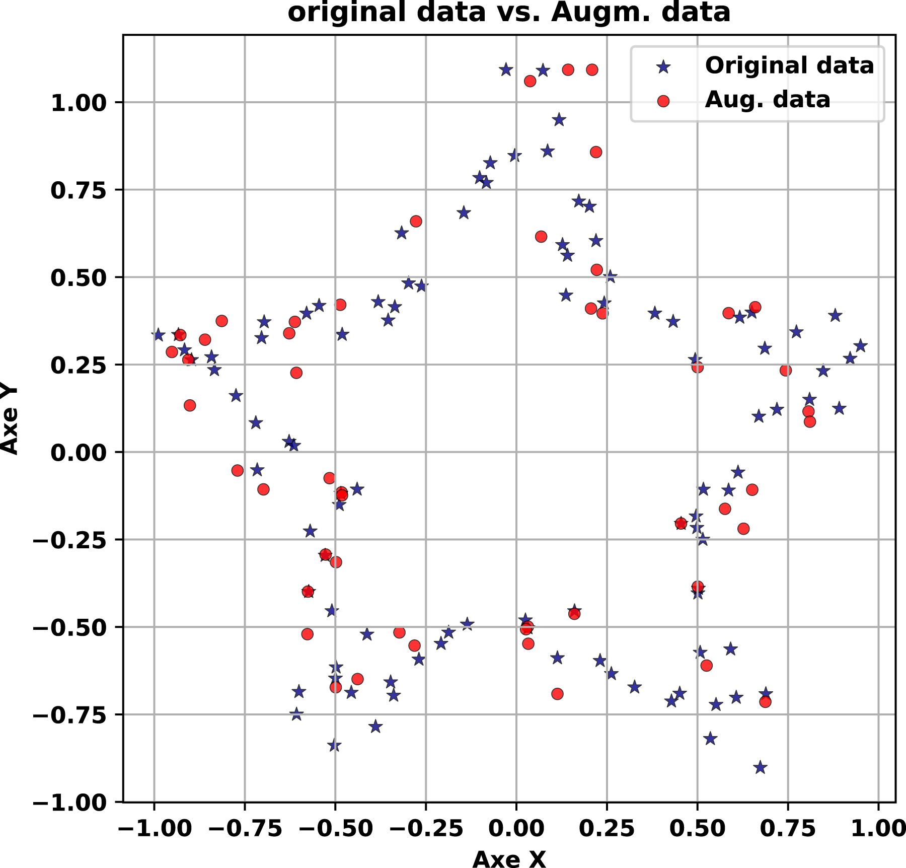
Figure 4: Generated vs. original star shape (Noise level = 5).
Next, we generate synthetic data with a minimal noise level of 0.1, overlaid in red on the original dataset (blue) in Fig. 3.
The experiment concludes with synthetic data generated at a high noise level of 5.0, shown in red alongside the original (blue) in Fig. 4. Here, the synthetic points exhibit greater dispersion, spreading outward from the star’s arms in a cloud-like pattern. Despite this variability, the five-armed structure remains discernible, with each arm still traceable amid the noise. This outcome highlights the generator’s robustness: it introduces significant diversity while retaining the core geometric essence of the original dataset. The trade-off between variability and fidelity is evident, as the increased noise broadens the synthetic distribution but does not obliterate the underlying pattern. This adaptability makes the method suitable for scenarios where controlled diversity is beneficial, such as data augmentation for machine learning, while still anchoring the synthetic output to the original structure.
Multiple Forms dataset experiment
The second synthetic experiment targets the Multiple Forms dataset, a more complex collection of 200 points distributed across four distinct shapes: a crescent, a circle, an asterisk, and a Gaussian cloud. This experiment, visualized in Fig. 5, tests the generator’s ability to handle multi-modal probability distributions with overlapping and diverse patterns.
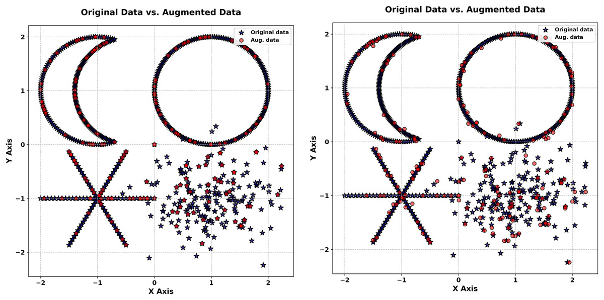
Figure 5: Generated vs. original star shape (Noise level = 0.1).
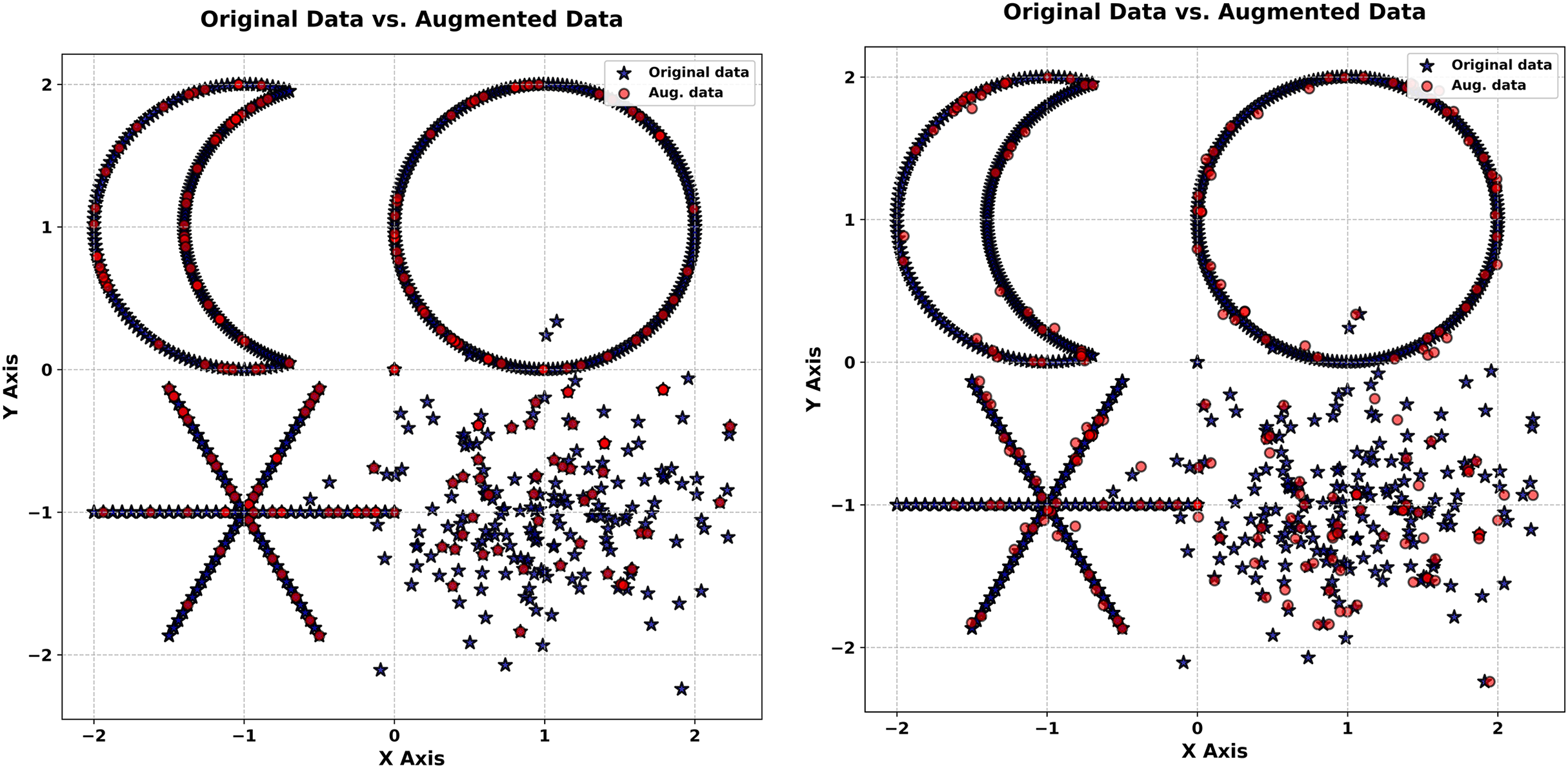
The experiment starts with Fig. 5 (right-hand), a scatter plot of the original dataset. The crescent’s smooth curvature, the circle’s closed boundary, the asterisk’s radial arms, and the Gaussian cloud’s dense cluster are all distinctly visible. This diversity of forms poses a significant challenge, requiring the generator to capture multiple structural characteristics simultaneously. The clarity of each shape in the original data sets a high bar for the synthetic outputs, making this dataset an excellent test of the method’s versatility in replicating complex patterns.
In the next stage, synthetic data generated with a noise level of 0.01 is overlaid in red on the original (blue) in Fig. 5 (left-hand). The synthetic points replicate each shape with remarkable accuracy: the crescent’s curve remains intact, the circle’s outline is precise, the asterisk’s arms are sharply defined, and the Gaussian cloud’s density is consistent. This close correspondence underscores the generator’s ability to preserve intricate, multi-modal probability distributions under low noise. The synthetic data mirrors the original so closely that distinguishing between them visually is challenging, highlighting the method’s precision in capturing both the marginal probability distributions and spatial relationships of diverse forms. This level of detail is particularly valuable for applications requiring faithful reproduction of complex datasets, such as simulation studies or generative modeling.
In Fig. 5 (right-hand) synthetic data at a noise level of 5.0 (red) is plotted against the original (blue). The increased noise level introduces noticeable dispersion, with synthetic points spreading outward from each shape. Nevertheless, the core features persist: the crescent’s arc, the circle’s boundary, the asterisk’s radial pattern, and the Gaussian cloud’s concentration remain recognizable. This resilience under high noise demonstrates the generator’s capacity to maintain structural integrity despite significant perturbation. The synthetic data introduces variability that enriches the dataset without erasing its defining characteristics, a balance that enhances its utility for tasks like robustness testing or diversity-driven analysis.
Experiments on real-world datasets
Following the synthetic experiments, we shift to real-world datasets, which introduce practical complexities such as mixed data types, varying sample sizes, and high-dimensional feature spaces. The experiments proceed in sequence across the Adult, Ecoli, Forest Fires, and Wisconsin Diagnostic Breast Cancer (WDBC) datasets, with analyses tied to Figs. 6–13.
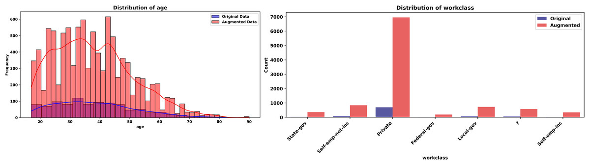
Figure 6: Correlation heatmap (Adult dataset, original vs. augmented).
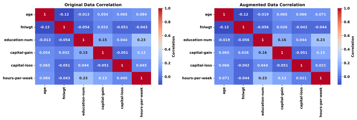
Figure 7: Correlation heatmap (Ecoli dataset, original vs. augmented).
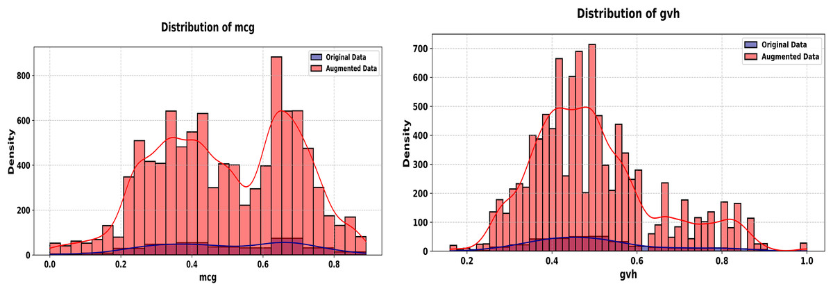
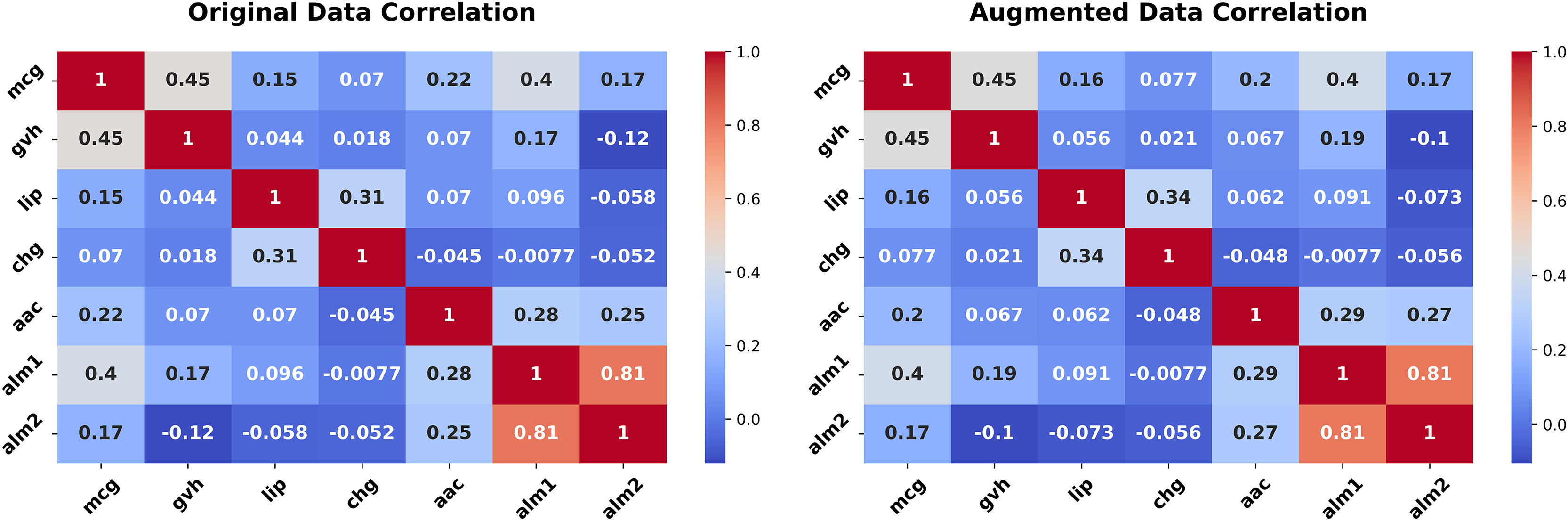
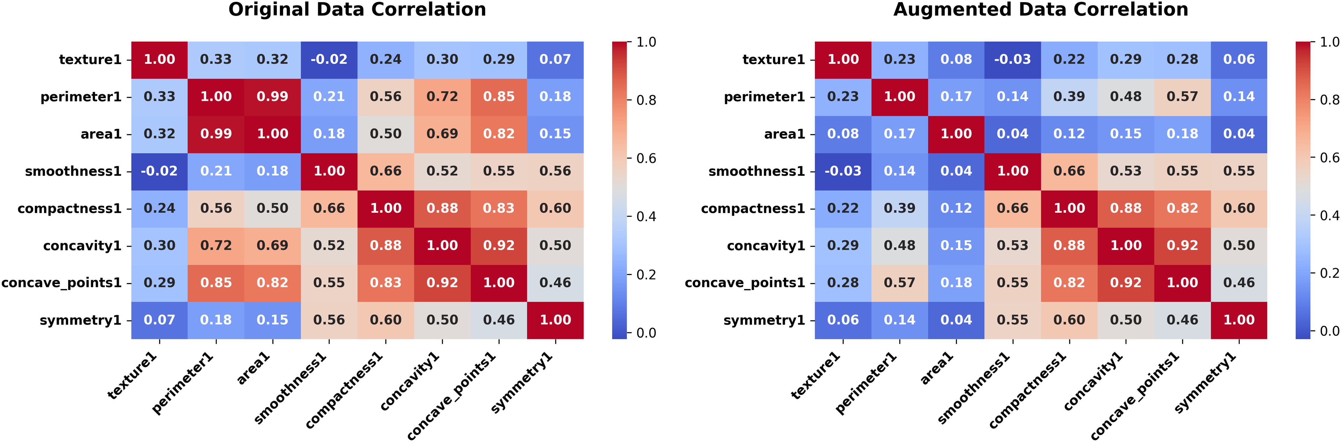
Figure 8: Correlation heatmap (WDBC dataset, original vs. augmented).
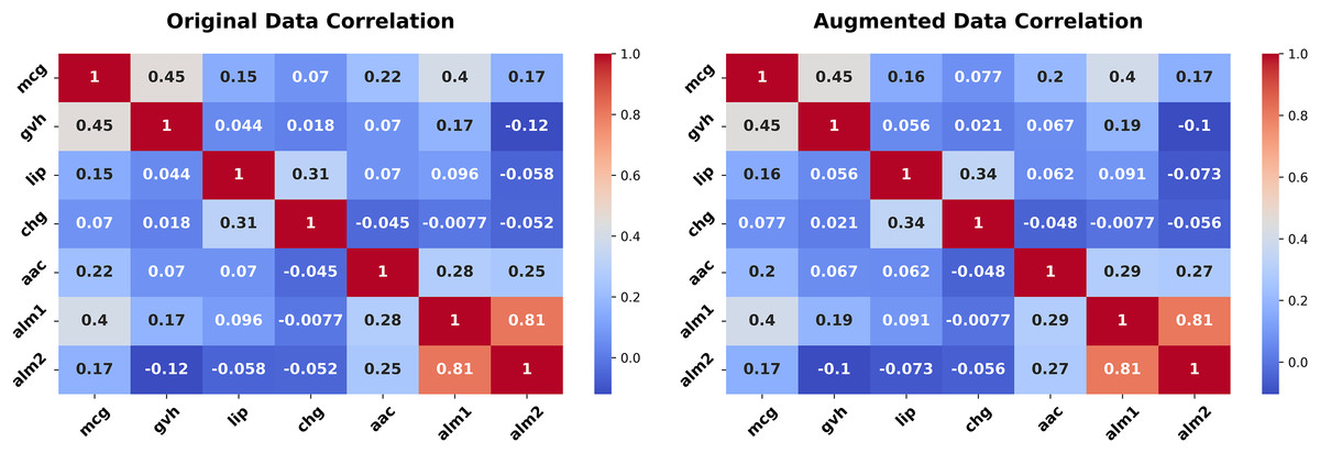
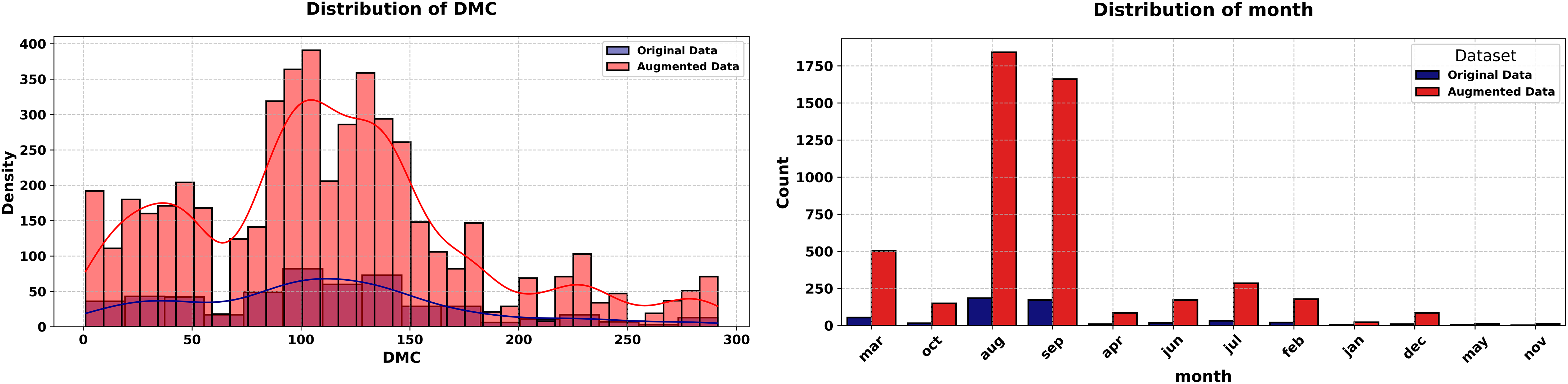
Figure 9: Histograms of Duff Moisture Code (DMC) and month features (Forest Fires dataset, original vs. augmented).
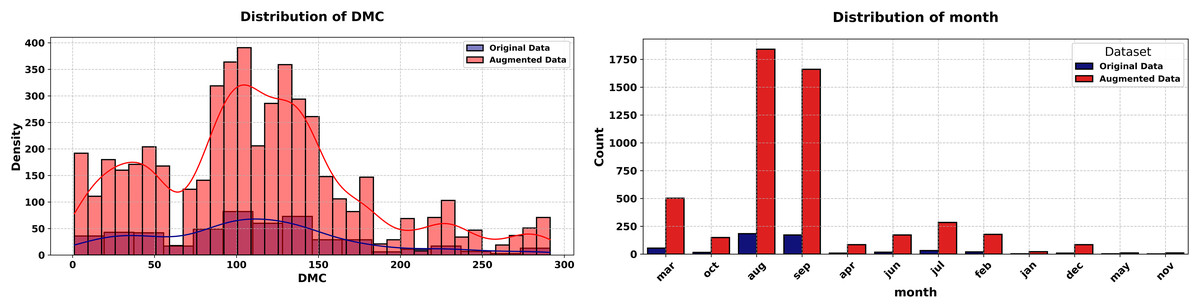
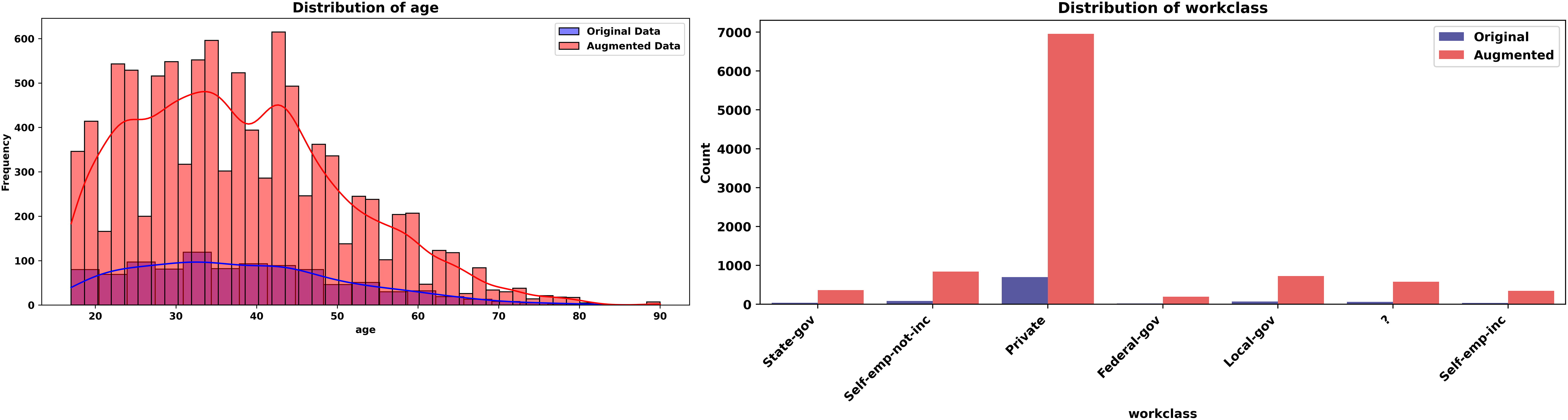
Figure 10: Histograms of age and workclass (Adult dataset, original vs. augmented).
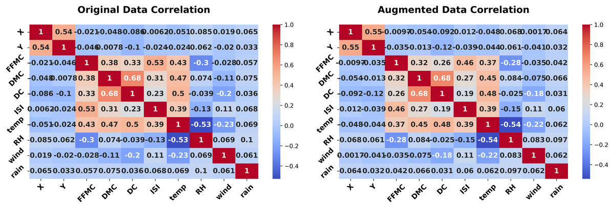
Figure 11: Histograms of mcg and gvh features (Ecoli dataset, original vs. augmented).
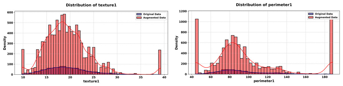
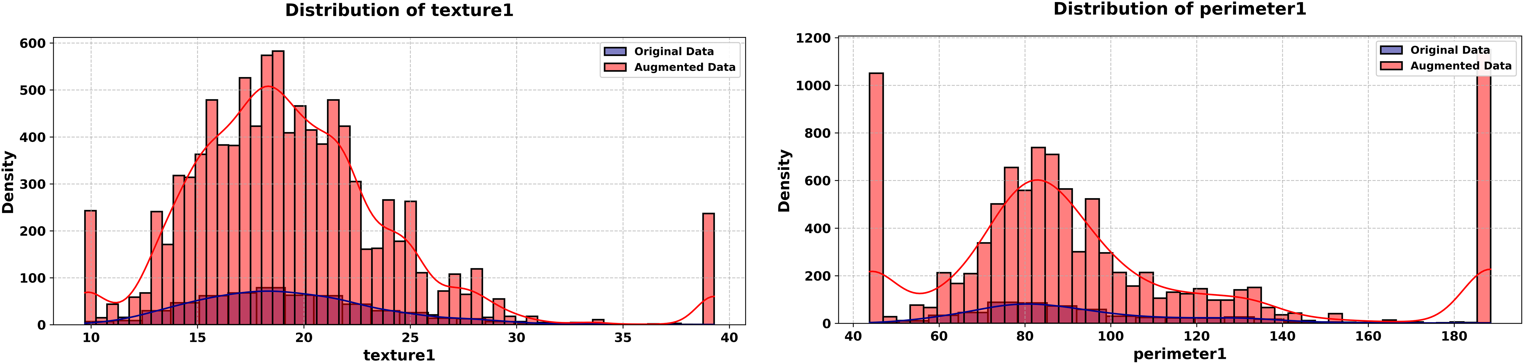
Figure 12: Histograms of texture 1 and perimeter 1 features (WDBC dataset, original vs. augmented).
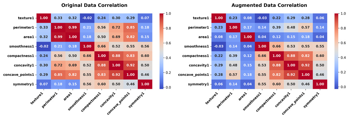
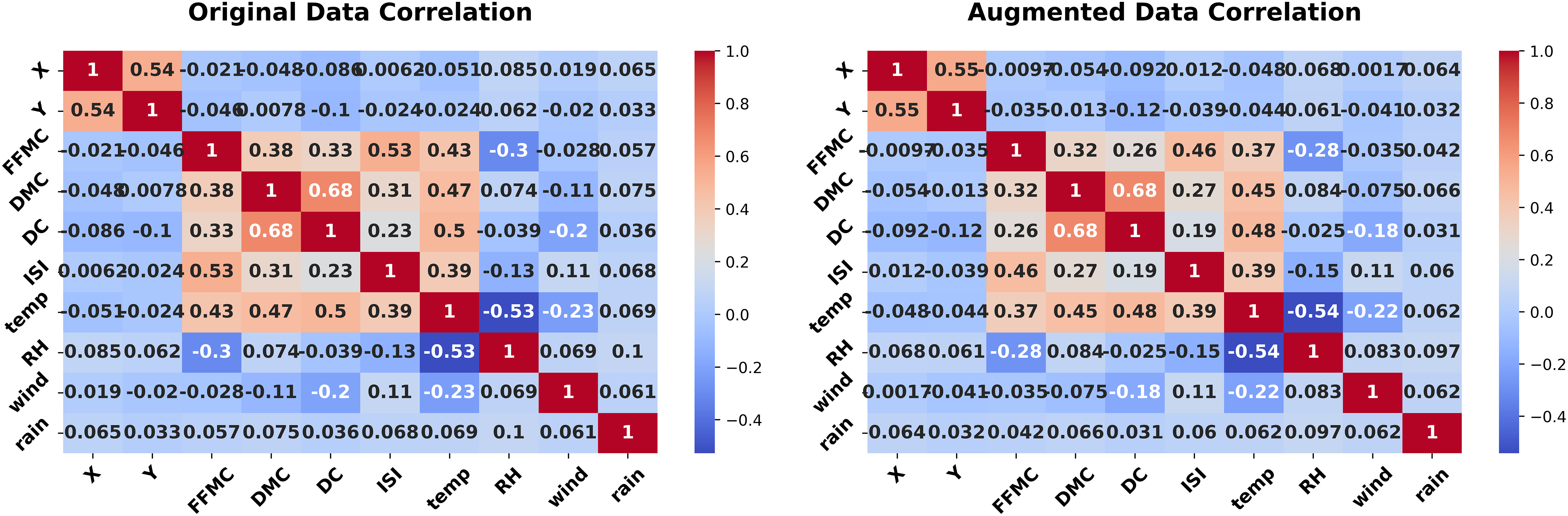
Figure 13: Correlation heatmap (Forest Fires dataset, original vs. augmented).
Adult dataset experiment
The Adult dataset is a widely used benchmark dataset in the field of machine learning and data science. Based on 1,000 records from this dataset and using 6 numeric and eight categorical features, we will generate 5,000 new records mimicking the original dataset using a level noise of 0.01. The experiment unfolds across Figs. 6, 7 for some features. The evaluation leverages the Kolmogorov-Smirnov (KS) test for numeric features, Jensen-Shannon (JS) divergence for categorical features and overall joint probability distributions, and correlation heatmaps for dependency structures
The experiment begins with Fig. 6 (left-hand), comparing histograms of the “age” feature from the original (blue) and synthetic (red) datasets. The probability distributions align closely, with the synthetic histogram replicating the original’s shape, peaks, and spread. A KS statistic of 0.0084 and p-value of 1.0000 indicate no significant difference, confirming the generator’s accuracy in preserving this numeric feature’s marginal probability distribution. Figure 6 (right-hand), quantifies the similarity of the categorical “workclass” feature using a JS divergence of 0.0107. This low value—close to 0, the ideal for identical probability distributions reflects the synthetic data’s ability to mirror the original frequency distribution across workclass categories (e.g., private, self-employed).
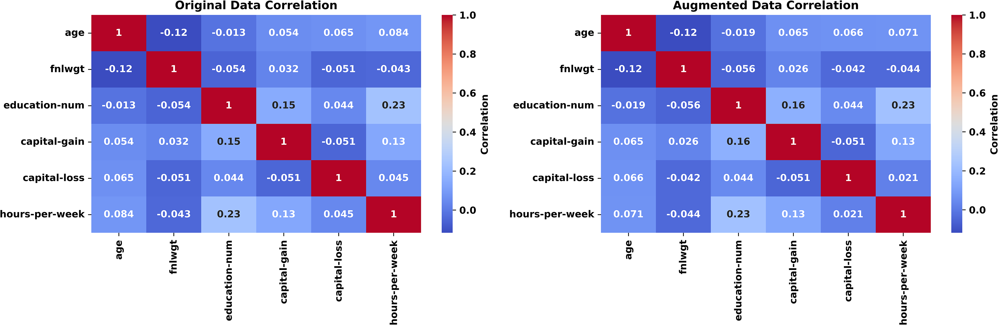
The experiment concludes with Fig. 7, presenting correlation heatmaps for the numeric features. The original (left) and synthetic (right) heatmaps are nearly indistinguishable, with correlation coefficients differing by less than 0.05 on average. Features like age and hours-per-week retain their interrelationships, demonstrating the generator’s success in capturing joint dependencies. This preservation is essential for applications where feature interactions inform outcomes, such as income prediction. The average JS divergence for the two datasets is insignificant (0.0117).
The Adult experiment (Figs. 6, 7) highlights the generator’s prowess with mixed-type data. Figure 5 confirms marginal fidelity for both examples: Numeric feature (age) and categorical feature (work class). Figure 6 validates joint fidelity for numeric features through the correlation heatmap. The low KS and JS metrics, paired with consistent correlations, highlight the method’s robustness in demographic contexts, where both individual and relational properties must be accurately replicated.
Ecoli dataset experiment
The Ecoli dataset involves 336 records with seven continuous predictor features. The proposed method synthesizes 5,000 new records that replicate the statistical properties of the original dataset, incorporating a noise parameter of 0.01 to introduce controlled variability. The experiment unfolds across Figs. 8, 9 for some features. The evaluation leverages the Kolmogorov-Smirnov (KS) test for numeric features, Jensen-Shannon (JS) divergence for categorical features and overall joint distributions, and correlation heatmaps for dependency structures.
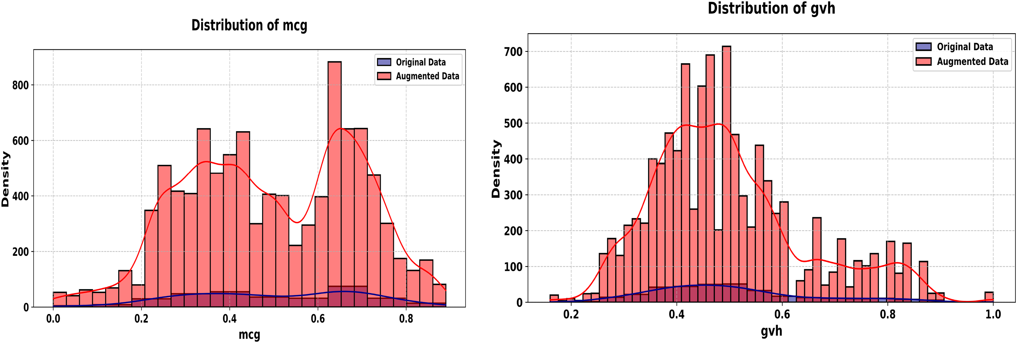
The experiment starts with Fig. 8, comparing histograms of the “mcg” and “gvh” features. The original (blue) and synthetic (red) distributions overlap tightly, with a KS statistic of 0.0174 and p-value of 1.0000 for the mcg feature and a KS statistic of 0.0073 and p-value of 1.0000 for gvh feature, indicating statistical equivalence. This precision in replicating a continuous feature’s probability distribution is vital for biological datasets, where small sample sizes amplify the importance of fidelity.
In Fig. 9, we show the correlation heatmaps for all numeric features. The original (left) and synthetic (right) heatmaps align closely, with minimal deviations in correlations among features like mcg and gvh. This consistency underscores the generator’s ability to preserve joint dependencies, critical for scientific analyses relying on inter-feature relationships.
The average JS divergence for the two datasets is insignificant (0.0134). The Ecoli experiment (Figs. 8, 9) demonstrates the generator’s effectiveness in small, continuous datasets. Figure 8 affirms the marginal fidelity, while Fig. 9 confirms joint fidelity. The low KS statistics and consistent heatmaps highlight the method’s utility in data-scarce scientific domains, where precision is paramount.
Forest Fires dataset experiment
The Forest Fires dataset experiment with 517 records, 10 numeric features, and two categorical features, assesses the generator on environmental data with temporal elements. The proposed method synthesizes 5,000 new records that replicate the statistical properties of the original dataset, incorporating a noise parameter of 0.01 to introduce controlled variability. The experiment begins with Fig. 10 (left-hand), comparing histograms of the Duff Moisture Code (DMC) feature. The original (blue) and synthetic (red) distributions are nearly identical, with a KS statistic of 0.012 and p-value of 1.0000. This fidelity ensures that key environmental indicators are preserved, supporting applications like fire risk modeling.
Figure 10 (right-hand), quantifies the similarity of the categorical “month” feature using a JS divergence of 0.0134 indicating high similarity between the original and synthetic distributions of this categorical variable. The low divergence preserves temporal patterns, essential for analyzing seasonal trends in environmental data. The experiment concludes with Fig. 11, presenting correlation heatmaps for numeric features. The original (left) and synthetic (right) heatmaps align closely, with features like DMC, temp, and wind showing consistent correlations. This preservation of dependencies enhances the synthetic data’s utility for environmental studies.
The experiment concludes with Fig. 11, presenting correlation heatmaps for numeric features. The original (left) and synthetic (right) heatmaps align closely, with features like DMC, temp, and wind showing consistent correlations. This preservation of dependencies enhances the synthetic data’s utility for environmental studies. The low KS and JS metrics, paired with consistent correlations, affirm the method’s robustness in practical settings.
Wisconsin Diagnostic Breast Cancer dataset experiment
The final experiment targets the Wisconsin Diagnostic Breast Cancer (WDBC) dataset, It contains 569 records and 29 continuous features, testing the generator in a high-dimensional medical context. The experiment unfolds across Figs. 12, 13 for some features.
The proposed method synthesizes 5,000 new records that replicate the statistical properties of the original dataset, incorporating a noise parameter of 0.001 to introduce controlled variability.
The experiment starts with Fig. 12, comparing histograms of the “texture1” feature. The original (blue) and synthetic (red) istributions align closely, with a KS statistic of 0.0118 and p-value of 1.0000, confirming marginal fidelity in a high-dimensional setting, it continues with the “perimeter1” feature, where the synthetic distribution matches the original (KS statistic = 0.0126, p-value = 1.0000). This consistency across features highlights the generator’s scalability to high-dimensional data.
In the WDBC dataset, the ECG achieved an average JS divergence of 0.0292 between the original and synthetic datasets. This exceptionally low value highlights the method’s proficiency in replicating the intricate statistical structure of a 29-feature dataset, with minimal deviations that affirm its robustness for high-dimensional applications. Correlation heatmaps show that features align closely (Fig. 13).
Dataset complexity effect on augmentation data quality
The quality of augmented data hinges on factors like the noise level, controlled by the noise level epsilon, and the Q ratio, calculated as the number of records divided by the number of features, which reflects the dataset’s informational density. Across four real-world datasets: Adult, Wisconsin Diagnostic Breast Cancer (WDBC), Ecoli, and Forest Fires, we see clear trends in how these elements shape the preservation of feature distributions. In the Adult dataset, boasting a high Q ratio of 71, the augmentation shines in Table 1, representing lower and higher noise levels, respectively. For continuous features like “age,” the KS statistic barely budges (0.0112 for ε = 0.01, 0.0120 for ε = 5), with p-values holding steady at 0.999, signaling robust similarity despite rising epsilon. Categorical features, such as “workclass,” also fare well, with JSD shifting only slightly from 0.0065 to 0.0093, hinting that a high Q ratio acts as a shield against noise, preserving fidelity across conditions. In contrast, the WDBC dataset, with a leaner Q ratio of 19.62, struggles as noise escalates. Table 2 shows “perimeter1” closely aligned (KS = 0.0151, p = 0.9997) for ε = 0.001, but reveals a stark drop-off (KS = 0.1088, p = 0) for ε = 0.01, exposing how low Q ratios leave datasets vulnerable to distributional drift under higher noise. The Ecoli dataset, sitting at a moderate Q ratio of 48, strikes a middle ground—Table 3 reports “mcg” with a KS of 0.0125 and p-value of 1.0000 for ε = 0.01, it rises to 0.0441 for ε = 5, yet retains a p-value of 0.5577, suggesting resilience that does not quite match the consistency of the Adult dataset. Likewise, the Forest Fires dataset, with a Q ratio of 43.08, displays varied outcomes: “DMC” in Table 4 holds tight (KS = 0.0150, p = 0.9999) for ε = 0.01, but “FFMC” diverges sharply (KS = 0.4717, p = 0) for ε = 1, though categorical “month” stays stable (JSD = 0.0141 and 0.0117), unsurprising since noise targets only continuous features. Together, these patterns reveal that higher Q ratios bolster robustness against noise, while lower ratios amplify sensitivity, particularly for continuous features under larger epsilon values, offering practical guidance for applying the augmentation method effectively.
| noise scale ε = 0.01 | |||
|---|---|---|---|
| Feature | Type | KS Statistic/JSD | P-value |
| age | Cont | 0.0112 | 0.9999 |
| fnlwgt | Cont | 0.0124 | 0.9994 |
| education-num | Cont | 0.0074 | 1.0000 |
| capital-gain | Cont | 0.0036 | 1.0000 |
| workclass | Cat | 0.0065 | – |
| education | Cat | 0.01964 | – |
| marital-status | Cat | 0.0090 | – |
| noise scale ε = 5 | |||
|---|---|---|---|
| Feature | Type | KS Statistic/JSD | P-value |
| age | Cont | 0.0120 | 0.9997 |
| fnlwgt | Cont | 0.0136 | 0.9976 |
| education-num | Cont | 0.0044 | 1.0000 |
| capital-gain | Cont | 0.0066 | 1.0000 |
| workclass | Cat | 0.0093 | – |
| education | Cat | 0.0209 | – |
| marital-status | Cat | 0.0101 | – |
| noise scale ε = 0.001 | ||
|---|---|---|
| Feature | KS Statistic | P-value |
| texture1 | 0.0129 | 1.0000 |
| perimeter1 | 0.0151 | 0.9997 |
| area1 | 0.0378 | 0.4453 |
| smoothness1 | 0.0104 | 1.0000 |
| noise scale ε = 0.01 | ||
|---|---|---|
| Feature | KS Statistic | P-value |
| texture1 | 0.0222 | 0.9568 |
| perimeter1 | 0.1088 | 0 |
| area1 | 0.3286 | 0 |
| smoothness1 | 0.0135 | 1.0000 |
| noise scale ε = 0.01 | ||
|---|---|---|
| Feature | KS Statistic | P-value |
| mcg | 0.0125 | 1.0000 |
| gvh | 0.0124 | 1.0000 |
| lip | 0.0020 | 1.0000 |
| chg | 0.0008 | 1.0000 |
| noise scale ε = 5 | ||
|---|---|---|
| Feature | KS Statistic | P-value |
| mcg | 0.0441 | 0.5577 |
| gvh | 0.0647 | 0.1367 |
| lip | 0.0106 | 1.0000 |
| chg | 0.0012 | 1.0000 |
| noise scale ε = 0.01 | |||
|---|---|---|---|
| Feature | Type | KS Statistic/JSD | P-value |
| FFMC | Cont | 0.0469 | 0.2464 |
| DMC | Cont | 0.0150 | 0.9999 |
| DC | Cont | 0.0181 | 0.9973 |
| ISI | Cont | 0.0101 | 1.0000 |
| month | Cat | 0.0141 | – |
| Day | Cat | 0.0120 | – |
| noise scale ε = 1 | |||
|---|---|---|---|
| Feature | Type | KS Statistic/JSD | P-value |
| FFMC | Cont | 0.4717 | 0 |
| DMC | Cont | 0.1031 | 0.0001 |
| DC | Cont | 0.4323 | 0 |
| ISI | Cont | 0.0170 | 0.9989 |
| month | Cat | 0.0117 | – |
| Day | Cat | 0.0103 | – |
Comprehensive synthesis and implications
Across all experiments, the ECG exhibits the following:
Marginal fidelity: Low KS statistics (0.0073–0.0174) and JS divergences (0.0107–0.0134) across datasets.
Joint fidelity: Consistent heatmaps, with minor challenges in high-dimensional cases (Wisconsin).
Noise flexibility: Synthetic experiments (Figs. 2–5) show adaptability from precision to variability. Bounded noise perturbation procedure ensures stable outputs across varying levels (0.01 to 5.0) except for leaner ratio.
Versatility: Success across synthetic and real-world contexts.
Limitations include computational scalability for extremely large datasets, an aspect that does not compromise its statistical precision but suggests potential for optimization, suggesting areas for future enhancement. In high-dimensional settings with a low sample-to-feature ratio, the ECG faces significant challenges. However, this difficulty is not unique to the generator; it reflects a broader issue in data analysis where the limited number of data points fails to fully capture the underlying probability distribution of the data. Nonetheless, this extensive evaluation confirms the generator’s broad applicability for synthetic data generation.
Computational complexity and empirical runtime evaluation
To investigate the scalability and efficiency of our proposed framework, we analyze the computational complexity of each stage in the pipeline. The full process consists of three main components: transforming the marginals to a uniform domain, generating synthetic samples from the copula-defined dependence structure, and inverting the synthetic samples back to the original data space. Each of these steps incurs specific computational costs, which depend on the number of features, original samples, and synthetic points. We detail these complexities below to highlight the algorithm’s performance characteristics and identify the dominant operations in practical use cases. In fact the proposed framework operates in three sequential stages: The first stage transforms each marginal feature into the uniform domain via empirical cumulative distribution functions (ECDFs). This requires sorting each feature column, which has a worst-case complexity of O(n. log (n)) per feature. Hence, for d features, the total complexity of this transformation is O(d.n .log (n)).
In the second stage, we generate m synthetic samples from the copula model defined over the uniform marginals. This process involves sampling from a dependence structure (e.g., Gaussian or empirical copula) and has linear complexity O(d⋅m), assuming constant-time sampling per dimension.
The third and final stage inverts the synthetic uniform samples back into the original data space using interpolation over the inverse ECDFs. Since each synthetic point is transformed dimension-wise, this stage also exhibits a linear cost of O(d⋅m). Aggregating all stages, the total runtime complexity of the full pipeline becomes:
which simplifies to O(d⋅m) in high-throughput settings where synthetic data generation dominates (i.e., m ≫ n).
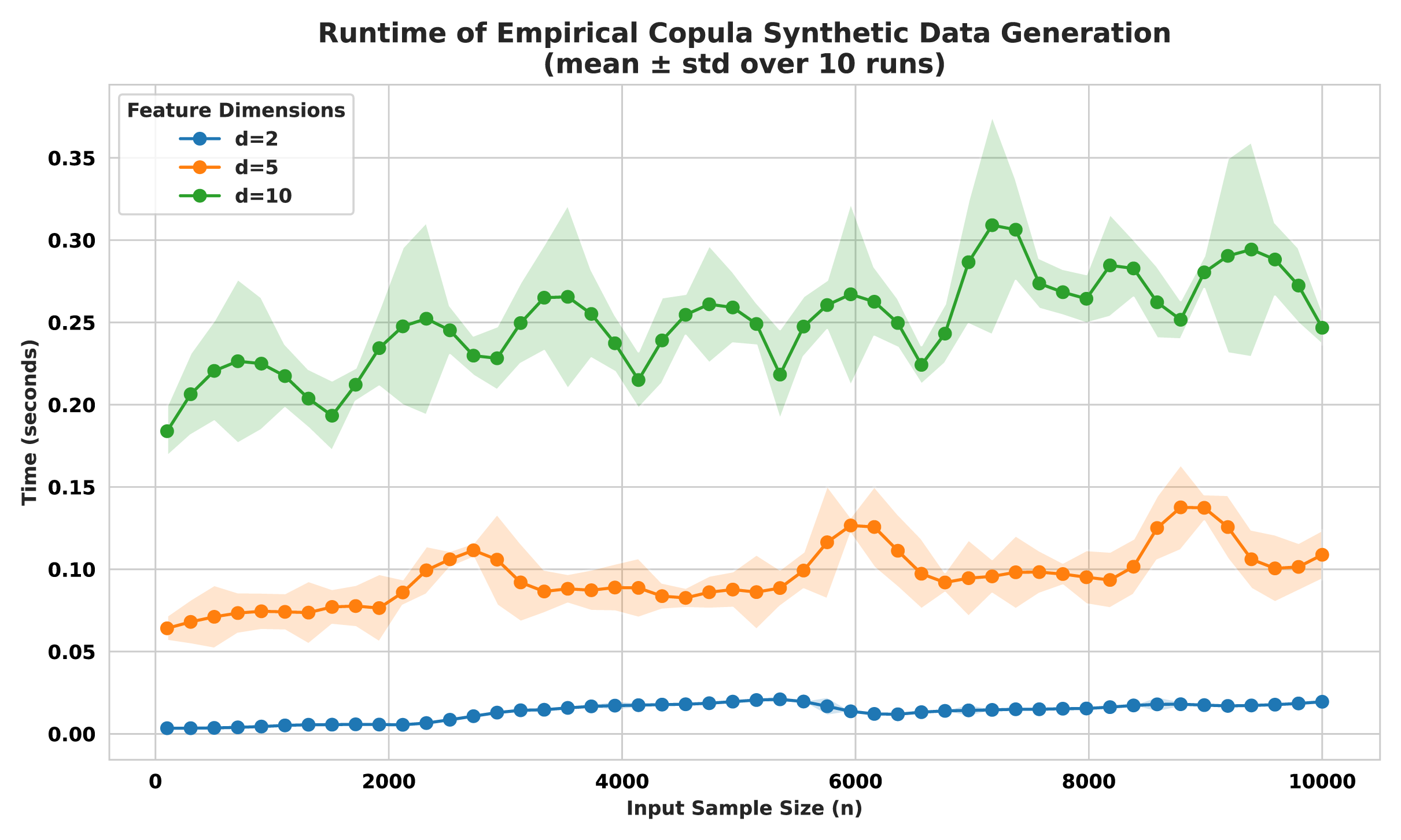
Runtime assessment on synthetic and real-world mixed-type datasets
Empirical runtimes obtained from a random (n,d) sample with the three mixed types are visualized in Fig. 14. The plot clearly demonstrates the expected linear scaling of computation time with respect to sample size n, across all three-feature dimensions. Additionally, increasing the number of features d results in proportional increases in runtime, validating the multiplicative role of dimensionality in the algorithm. Importantly, no super-linear behavior was observed, confirming the framework’s suitability for efficient augmentation in large-scale, mixed-type datasets.
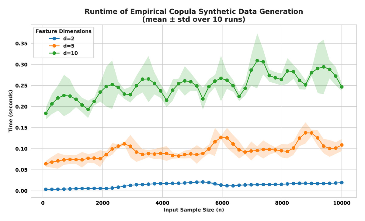
Figure 14: Multiple forms dataset generated with a noise level of 0.01 and 5.0.
The benchmark experiment conducted here consists of using three mixed-type synthetic datasets. Each dataset composed of a combination of (i) continuous features drawn from Gaussian or uniform distributions, (ii) ordinal features mimicking ordered categories, and (iii) nominal categorical features representing non-ordered classes type. All categorical and ordinal variables were preprocessed using appropriate encoding schemes to allow unified treatment. We systematically varied the number of features d ∈ {2, 5, 10} while incrementing the sample size n ∈ [100, 10,000] uniformly to assess the computational impact of both data dimensionality and original sample size.
Furthermore, the runtime performance of our empirical copula-based data generation approach was evaluated across multiple datasets and varying feature dimensions. We measured the average generation time for producing 10,000 synthetic samples (averaged over 100 runs) using four benchmark datasets. For the Adult dataset (1,000 samples, 10 features), the mean execution time was 0.192 s. The Ecoli dataset (336 samples, eight features) required 0.137 s, while the Forest Fires dataset (517 samples, 12 features) took 1.2036 s. The most computationally intensive case was the WDBC dataset (569 samples, 30 features), reaching 5.1162 s. These results confirm that the method is efficient and scalable for low and high dimensional data (refer to Endres, Mannarapotta Venugopal & Tran (2022) to compare with other methods).
Empirical assessment of downstream model gain
To evaluate the effectiveness of our proposed data augmentation method under low-data conditions, we conducted a series of 20 independent trials using the Adult dataset from the UCI Machine Learning Repository. In each trial, we randomly sampled only 2% of the full dataset (455 training instances), simulating a realistic low-resource scenario. The goal was to determine whether augmenting this small subset with 5,000 synthetically generated samples created using our empirical copula-based method tailored for mixed (categorical and continuous) data could significantly improve downstream classification performance. We trained a Random Forest classifier using both the original limited dataset and the augmented version, and evaluated performance on a held-out test set.
The results show a consistent and meaningful improvement in both classification accuracy and F1-score across all trials. Without augmentation, the model achieved a mean accuracy of 0.8048 (±0.0187) and a mean F1-score of 0.4562 (±0.0789). With our data augmentation applied, the accuracy increased to 0.8317 (±0.0161), and more importantly, the F1-score improved substantially to 0.5676 (±0.0715). This uplift in F1-score despite a marginal gain in overall accuracy indicates that the augmented data significantly improved the model’s ability to correctly identify the minority class, which is particularly valuable in the presence of class imbalance. These findings highlight the robustness and effectiveness of our method in enhancing classifier performance under constrained data availability.
The code, plots, and results associated with this work are publicly available on our GitHub repository and Zenodo (https://github.com/mohsenbenhassine/data-augmentation; DOI 10.5281/zenodo.17288914).
Broader implications, challenges, and future directions
In this section, we discuss the broader implications of our work on the ECG, a method designed to generate synthetic data that preserves the statistical properties of original datasets. We highlight the challenges encountered during the study, outline potential avenues for future research, and propose directions to enhance the scalability and versatility of our approach.
The ECG represents a significant advancement in synthetic data generation, offering a robust and non-parametric method to create realistic datasets that maintain the statistical integrity of the original data while ensuring privacy. This capability has profound implications across multiple domains where data privacy is a critical concern, such as healthcare, finance, and social sciences. For instance, in healthcare, the generator can produce synthetic patient records that mirror real probability distributions and dependencies, enabling researchers to share and analyze data without risking individual privacy breaches. Similarly, in finance, it can facilitate the development of models using synthetic datasets that comply with regulatory requirements.
Beyond privacy-preserving applications, our method enhances machine-learning workflows by providing augmented datasets for training models (Sawada et al., 2025), particularly in cases where real data is scarce, imbalanced, or difficult to obtain. The ability to generate diverse yet statistically consistent datasets also supports robustness testing and validation of machine learning models, ensuring they perform reliably across varied scenarios. By bridging the gap between data availability and statistical fidelity, the ECG positions itself as a versatile tool with the potential to accelerate innovation in data-driven fields. Our proposed ECG method demonstrated significant improvements in both computational efficiency and downstream predictive performance. Compared to the methods in Endres, Mannarapotta Venugopal & Tran (2022), ECG achieved substantially lower runtime, particularly in high-dimensional settings, as shown in our complexity analysis and runtime benchmarks. Beyond speed, ECG also led to notable gains in downstream model performance, yielding consistently higher accuracy and F1-scores when evaluated on real-world classification tasks. These results confirm that ECG not only scales efficiently but also produces high-quality synthetic data that effectively enhances model learning, especially in low-resource and imbalanced data scenarios.
While the ECG demonstrates strong performance across various datasets, our study revealed several challenges that underscore areas for improvement. One prominent challenge was its performance in high-dimensional settings. Addressing computational efficiency is vital for large-scale applications; parallelized or distributed implementations on graphics processing unit (GPU) clusters or cloud platforms could substantially cut processing times. This issue highlights the need for refinements to ensure the method remains effective in larger feature spaces. To address the identified challenges and further enhance the scalability and versatility of the ECG, we propose several avenues for future research. First, improving the method’s ability to handle high-dimensional data with non-linear relationship could involve exploring advanced copula statistics as Copula Statistic (CoS) index (Hassine, Mili & Karra, 2017) or dimensionality reduction techniques. Leveraging machine-learning techniques within Vine Copulas or applying block-wise augmentation , encoders or neural networks in general, could better capture non-linear dependencies, enhancing the generator’s accuracy in complex datasets. Second, optimizing computational efficiency is critical for scaling the method to big data scenarios. Developing parallelized or distributed versions of the algorithm could significantly reduce processing time, making the generator feasible for large-scale applications. This could involve adapting the method to run on modern computing frameworks, such as GPU or tensor processing unit (TPU) clusters or cloud-based platforms.
Finally, extending the ECG to accommodate additional data structures, such as time series (Iglesias et al., 2023) or graph data (Shorten & Khoshgoftaar, 2019) would significantly enhance its versatility. Many real-world applications involve temporal dynamics (e.g., stock prices) or relational structures (e.g., social networks), and adapting the method to these domains could open new opportunities for synthetic data generation. This might require incorporating temporal copulas or graph-based dependency models into the framework. Finally, a key future perspective involves rigorous comparisons with established methods like SMOTE, GANs, SDV-G, and VAEs to fully delineate the generator’s strengths and trade-offs. Benchmarking against these techniques using metrics such as JS divergence, Wasserstein distance, or downstream classification accuracy could quantify its superior preservation of mixed-type dependencies and highlight computational efficiency gaps, this could pave the way for hybrid innovations, such as merging the generator’s copula-based dependency modeling with GANs’ generative flexibility or VAEs’ latent space efficiency.