FEEL: fast and effective emotion labeling, a dual ensemble approach for effective facial emotion recognition
- Published
- Accepted
- Received
- Academic Editor
- Bilal Alatas
- Subject Areas
- Adaptive and Self-Organizing Systems, Artificial Intelligence, Data Mining and Machine Learning, Social Computing, Neural Networks
- Keywords
- Expressions, Emotions, Machine learning, Ensemble learning
- Copyright
- © 2025 Wang
- Licence
- This is an open access article distributed under the terms of the Creative Commons Attribution License, which permits unrestricted use, distribution, reproduction and adaptation in any medium and for any purpose provided that it is properly attributed. For attribution, the original author(s), title, publication source (PeerJ Computer Science) and either DOI or URL of the article must be cited.
- Cite this article
- 2025. FEEL: fast and effective emotion labeling, a dual ensemble approach for effective facial emotion recognition. PeerJ Computer Science 11:e3138 https://doi.org/10.7717/peerj-cs.3138
Abstract
Facial expressions are a vital channel for communicating emotions and personality traits, making automatic emotion recognition from facial images a task of growing importance with wide-ranging applications. While deep learning models have shown considerable promise in this domain, most existing approaches are unimodal and limited to classifying only six basic emotions. This study introduces a dual-ensemble deep learning framework designed to recognize both basic and complex blended emotions with high accuracy. The first ensemble focuses on detecting primary emotions using DenseNet-169, VGG-16, and ResNet-50 as base models. The second ensemble focuses on identifying nuanced emotional blends, utilizing Xception and vision transformer (ViT) architectures. A squeeze-and-excitation (SE) block is incorporated to emphasize the most salient features, thereby enhancing overall model performance. The proposed framework is trained and evaluated on the widely used Facial Expression Recognition (FER)2013 and Indonesian Mixed Emotion Dataset (IMED) datasets. Experimental results demonstrate its effectiveness, achieving 95% accuracy for basic emotion recognition and 88% for blended emotions. These findings underscore the potential of the proposed approach to advance human-computer interaction by improving both the accuracy and depth of automated emotion recognition systems.
Introduction
As social creatures, humans accompany facial expressions with verbal communication to properly convey their feelings. Along with consolidating communication, facial expression describes intentions and personality (De la Torre & Cohn, 2011). The basic emotions, as traced from facial expressions, are anger, disgust, surprise, happiness, fear, and sadness (Siedlecka & Denson, 2019; Ekman, 1999). However, there are mixed emotions besides the common ones, such as a bittersweet smile, a nostalgic look, and hopeful despair (Larsen & McGraw, 2011). Most of the research focuses on detecting and recognizing basic emotions. Formerly, statistical approaches were utilized to identify emotions from facial images (Londhe & Pawar, 2012; Neeru & Kaur, 2016). However, the accuracy of such systems was not up to the mark (Zhao & Zhang, 2015). Recent advancements in computer technology have enabled the precise identification and categorization of emotional states from input images. Machine learning (ML)-based systems have also been designed to learn and automatically detect facial expressions (Rahul & Ouarbya, 2023). As simple machine learning classifiers, such as support vector machine (SVM) and k-nearest neighbor (KNN), suffer from overfitting (Kopalidis et al., 2024); researchers prefer deep learning models for automated emotion recognition (Wei & Zhang, 2020; Mellouk & Handouzi, 2020). The unimodal systems in the literature target the universal emotion (Akeh & Kusuma, 2025), whereas the performance of no single deep learning model is optimal. Therefore, there is a need for an ensemble-based approach to accurately recognize both mixed and straightforward emotions, which motivates this research.
The implementation of a dual-stage strategy has been motivated by the need to handle diverse emotion categories more effectively. In this framework, the initial ensemble is designed to focus on recognizing fundamental emotions, while the secondary ensemble has been dedicated to classifying complex and blended expressions. By isolating the learning responsibilities, specialization is promoted at each stage, and challenges related to class overlap and ambiguity are better mitigated than in traditional single-stage models.
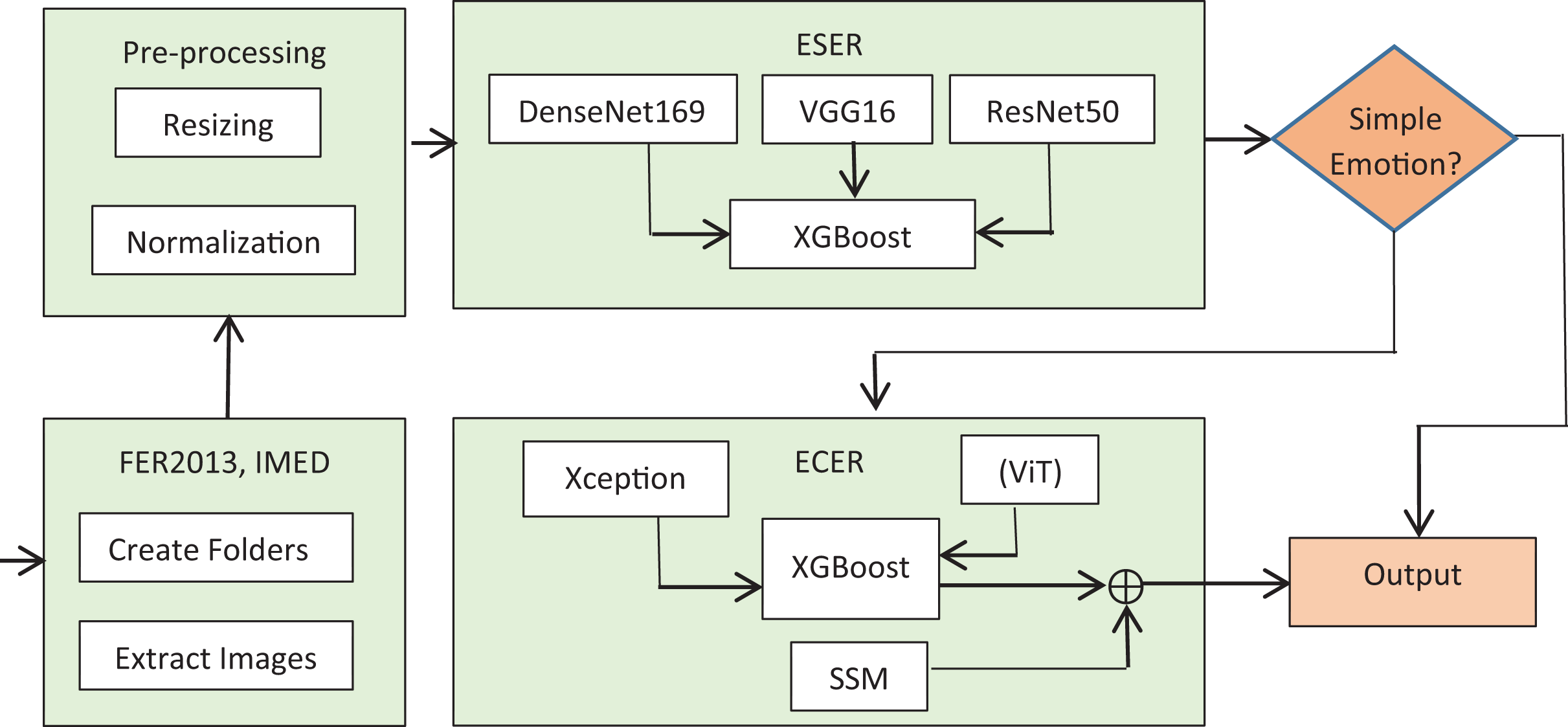
This study proposes a dual ensemble approach to detect common and blended emotions from input facial images. The method works in two phases. In the first phase, the Ensemble for Simple Emotion Recognition (ESER) model detects seven basic emotions. In the second phase, the Ensemble for Complex Emotion Recognition (ECER) model deals with recognizing blended emotions. The Facial Expression Recognition (FER)2013 and Indonesian Mixed Emotion (IMED) datasets (Akeh & Kusuma, 2025) are utilized for training, validation, and testing. The system starts with ESER and generates percentage prediction accuracies for the basic emotions. If the emotion conveyed by the input image is of a simple emotion, the corresponding class is predicted. If the emotion is not typical, further classification is performed by ECER at the second level. Besides direct classification by advanced deep learning classifiers, supporting statistics are examined in the secondary statistics module (SSM) for precise prediction. For operative training, the SE block is utilized to prioritize important features. In ESER, the DenseNet169 (Huang et al., 2017), VGG16 (Simonyan & Zisserman, 2014), and ResNet50 (He et al., 2016) are used as base models, whereas in ECER, the Xception (Chollet, 2017) and vision transformer (ViT) (Huo et al., 2023) are employed. The decision tree-based algorithm-eXtreme Gradient Boosting (XGBoost) (Ali et al., 2023) is used as a meta learner. Based on the meta-features fed to the XGBoost classifier, the correct type of emotion is predicted. For the optimal prediction of blended emotion, 60% weightage is paid to the ensemble-based recognition output, whereas 40% is paid to the mode’s statistics behind the emotion. The method is systematically evaluated and the outputs are analyzed from different perspectives. Results of the evaluations indicate that the method not only outperforms the individual models in terms of precision, recall, accuracy and F1-score but also detects blended emotions with commendable accuracy. Without the ensemble approach, the average accuracy for the basic emotions is 89%, whereas that of the mixed emotion traced is 70.45%. However, with an ensemble approach, the accuracy of detecting basic emotions increased to 95%, while that of the mixed emotions increased to 88.7%. This significant increase vividly shows that the framework is good for detecting various types of emotion and their significance in multiple domains, including security, health and education. Schematics of the proposed framework are shown in Fig. 1.
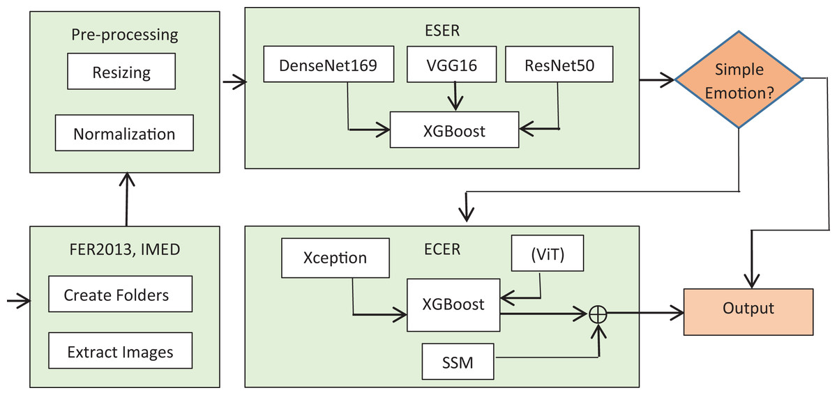
Figure 1: Schematic of the dual ensemble framework.
Figure 1: A schematic representation of the proposed dual-stage ensemble framework. In the first phase (ESER), primary emotions are classified, while in the second (ECER), complex blended emotions are recognized using both model predictions and secondary statistical support.
Related work
Facial expression recognition (FER) refers to identifying the states of human emotions from static images or videos. Some key information that is detectable from human face includes stress levels, boredom, confusion, and interest. Because of its wide range of applications in various fields like crime detection, health care, security, and augmented and virtual reality (Cai, Li & Li, 2023), several research works have been conducted to detect and recognize emotion effectively. As stated in Zhan et al. (2008), the market of emotion recognition is growing rapidly and will be projected to $136.2 billion by 2031. With the beginning of ML technology, expression recognition models were based on handcrafted features like histogram of oriented gradients (HOG) (Mohammadi, Khoury & Karray, 2014; Dalal & Triggs, 2005), local binary patterns (LBP) (Zhao & Zhang, 2011), and scale-invariant feature transform (SIFT) (Lowe, 2004). Support vector machines (SVM) and random forests have also been extensively utilized for emotion classification (Kremic & Subasi, 2015; Lajevardi & Wu, 2016). However, all such systems were light-sensitive, noise-dependent and suffered from various issues like pose and occlusion. The deep learning-based models, particularly convolutional neural networks (CNNs), are effective in FER (Fan, Lam & Li, 2020). The CNN architecture is followed in Lopes et al. (2017), Mollahosseini, Hasani & Mahoor (2017), Li, Huang & Luo (2018) are employed for temporal modeling. Hybrid approaches combining CNNs with other neural networks have also been exploited (Minaee, Azimi & Abdolrashidi, 2021; Ding, Zhou & Chellappa, 2020). Similarly, the RNN-based frameworks leverage spatial features besides temporal dependencies (Kahou et al., 2015; Fan, Lam & Li, 2018) for effective expression recognition. The YOLOv3-based system of Nafis, Navastara & Yuniarti (2020) recognizes facial expressions from real-time videos. The model gains 79% accuracy with 80% precision and 77% F1-score on the IMED dataset. Synthetic images to enhance FER via GAN are proposed in Wang (2021). However, as every individual model has some limitations, the research community prefers the ensemble approach. To contextualize the effectiveness of ML models, comparative analysis has also been presented in Kopalidis et al. (2024), highlighting recent approaches to facial emotion recognition in terms of architecture, performance, dataset usage, and support for blended emotions. Recent contributions from 2023 and 2024 have also explored the utility of ViT and lightweight CNNs in emotion recognition. Notably, hybrid transformer-CNN models and cross-attention architectures have been investigated for their efficiency and accuracy in handling complex emotional data (Zhang, Wang & Liu, 2023; Li, Sun & Huang, 2024; Khan et al., 2024).
Materials and Methods
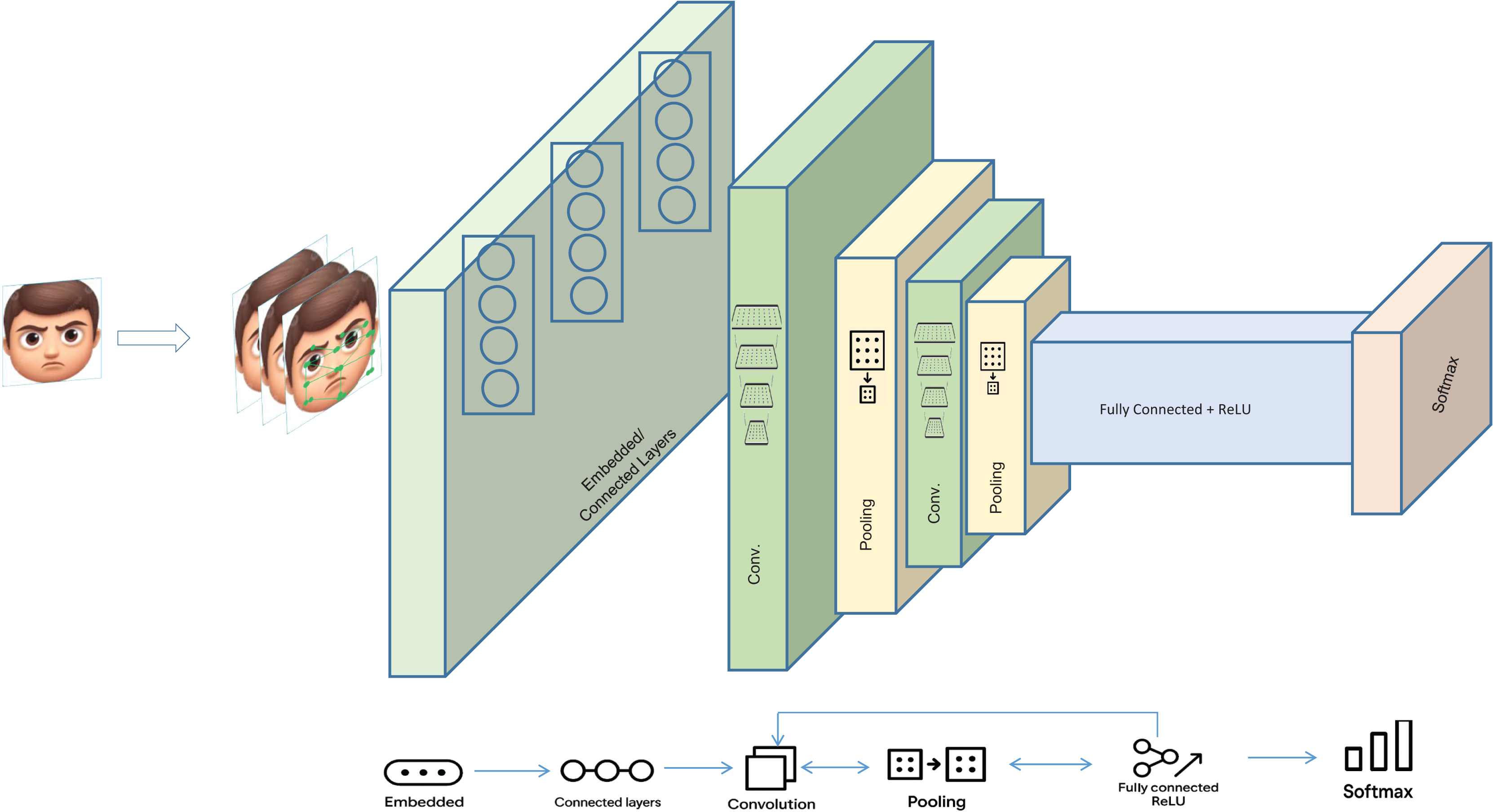
In this research work, a dual ensemble method is proposed to classify the typical and blended emotions accurately. As the functioning of no single FER model is optimal, an ensemble approach is utilized to have the cumulative potential of multiple models. The inadequacies of individual neural network models are overcome in the proposed method. Since the deep learning-based architecture- DenseNet169, VGG16, ResNet50, Xception, and ViT are effective in image classification, they are the base models. The XGBoost model is used as a meta-model to predict the correct emotion after extracting the complex relationships from the meta-features. The framework intends to offer improved accuracy with commendable generalization. The general working of the base models is illustrated in Fig. 2. All experiments were executed on a system configured with an AMD Ryzen 9 7950X processor, 64 GB DDR5 RAM, and an NVIDIA RTX 4090 GPU with 24 GB VRAM. Ubuntu 22.04 LTS served as the operating system. Deep learning tasks were implemented using TensorFlow 2.11 and PyTorch 1.13, while CUDA 11.8 and cuDNN 8.7 were used for GPU acceleration. Python 3.9 was employed for all scripting and model integration tasks.
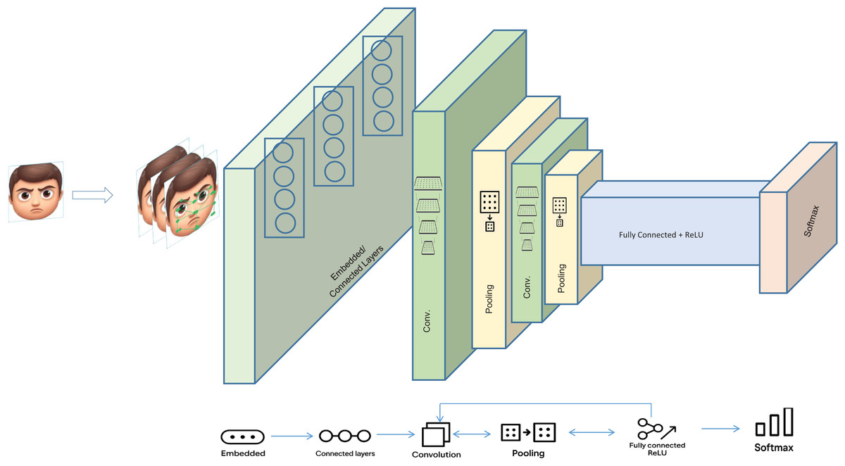
Figure 2: Working of the base models.
To effectively train and deploy the proposed framework, the following computing infrastructure is recommended:
1. Operating system (OS)
Preferred OS: Ubuntu 20.04+ (LTS) or Ubuntu 22.04 LTS
Optimized for deep learning and supports CUDA, cuDNN, and TensorFlow/PyTorch.
Better compatibility with GPU drivers and AI frameworks compared to Windows.
Alternative: Windows 11 with WSL2 (Windows Subsystem for Linux) for Linux-like flexibility on a Windows machine.
2. Hardware requirements
(a) Processor (CPU)
Recommended: AMD Ryzen 9 7950X/Intel Core i9-13900K
16+ cores, high multi-threading performance for pre-processing and data augmentation.
Supports efficient parallel processing for loading datasets and feature extraction.
(b) Graphics processing unit (GPU)
Primary choice: NVIDIA RTX 4090 (24 GB VRAM)/NVIDIA A100 (40 GB VRAM)
Essential for training ViT and CNN-based models (DenseNet, VGG16, ResNet50, Xception).
CUDA and cuDNN support to accelerate deep learning computations.
At least 24 GB VRAM recommended for large-scale training and ViT processing.
Alternative: NVIDIA RTX 3090 (24 GB) or NVIDIA RTX 4080 (16 GB) for slightly lower budget constraints.
(c) Memory (RAM)
Minimum: 32 GB DDR5
Recommended: 64 GB DDR5 or higher
Handles large image datasets (e.g., FER2013 and IMED) efficiently.
Supports multi-threaded data augmentation and batch processing without memory bottlenecks.
Preprocessing
From the Kaggle platform, the standard datasets-FER2013 are obtained besides the IMED. The IMED dataset, which contains images representing blended emotions, was annotated using a semi-supervised strategy. Initially, candidate labels were proposed using automated prediction thresholds from baseline classifiers. These were then verified and refined through manual review by three independent annotators. Each image label was finalized through majority voting. This ensured that the emotional labels represent plausible combinations recognized consistently by human reviewers. The dataset is available at https://www.kaggle.com/datasets/msambare/fer2013. The former dataset contains images of common facial expressions, while the latter is for blended emotions. Prior to training, the datasets are preprocessed to have all the images in the same size and shape. With the os library, seven folders are created for the common facial emotions. The CSV file contents are retrieved, and the image files are saved in their respective folders after the mat arrays are made. Normalization at the pixel level is performed to avoid overfitting and ensure generalization.
Normalization
The technique of z-score normalization is utilized to bring the pixel values of all input images into a standard range of 0 and 1. For pursuing the process, mean and standard deviation of the pixels of image are computed. A normalized image is obtained from an input image of channels ‘c’ with N pixels as,
(1) where,
(2)
(3)
In the equations, x and y represent the 2D positions of image pixels.
Image resizing
To bring all the images into the same standard size, images are resized. To preserve the pixels’ information while adjusting the dimensions, the scaling factor is ensured in every iteration. The factor for an input image with height and is given as, given as,
(4) where , represents the height and width of the resultant image
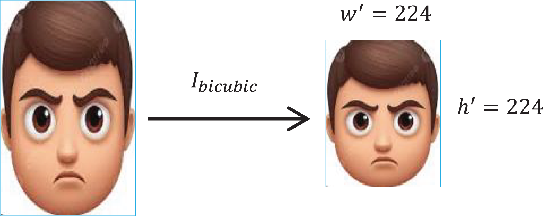
To retain the pixels’ intensity, the bicubic interpolation ( ) is applied, see Fig. 3. The operation is represented as,
(5)
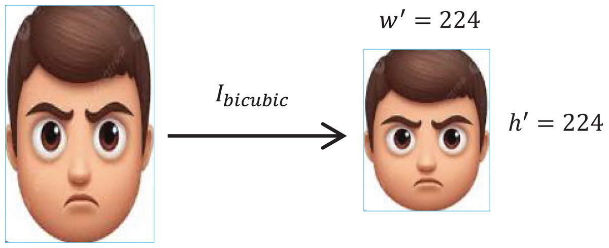
Figure 3: Image resizing with bicubic interpolation.
1st phase ensemble-ESER
In the 1st phase, the ESER model detects and recognizes basic emotions. The ensemble utilizes the three well-known CNN-based classifiers: DenseNet169, VGG16 and ReseNet50. After preprocessing, an unknown input image is passed through all the base models for prediction. As meta-features, the outputs of base models are fed to the meta-learner for precise recognition of emotion. The class of emotion for which the predicted accuracy score (PAS) of XGBoost is highest is supposed to be the class of input emotion. However, if the highest accuracy is less than 50%, the emotion is assumed to be blended. Therefore, the percent accuracies for sadness and happiness are stored in a separate CSV file-predicted mode in percent (PMP) for onward utilization in the second ensemble-ECER.
2nd phase ensemble-ECER
The secondary statistical module (SSM) serves as an auxiliary decision-support component that integrates emotion likelihoods from ESER into the ECER prediction process. It receives class-wise probabilities of happiness and sadness from the first ensemble and recalibrates the ECER output using predefined emotion distribution weights. This hybrid scoring approach, calculated using Eq. (6), is particularly effective when blended emotions exhibit shared traits with basic emotional patterns. Detection and recognition of complex emotions at the second level are done using the ECER model. Suppose more than two distinct classes are predicted in the first level and the accuracy of meta learner is below 50% in the first level. This will indicate that the image carries a complex emotion and needs to be further classified. In the second level of the ensemble, the Xception, ViT and DenseNet221 are utilized to recognize the blended emotion. DenseNet221 was incorporated in ECER due to its extended depth and improved gradient flow across layers. Compared to shallower variants, DenseNet221 facilitates more refined feature extraction in deeper layers, which is particularly advantageous when dealing with nuanced patterns typical of blended emotional states. Its inclusion was based on empirical testing, where it showed superior feature abstraction for complex emotion patterns. To avoid the possibility of false recognition, the direct recognition by the ECER is complemented by supporting statistics in the SSM module. The percentage scores of happiness and sadness (obtained from the PMP) are used in SSM. The explicit formula used for the precise detection of the correct complex emotion is designed such that to give 60% weightage to direct recognition and 40% to the statistics behind the blended emotion. The net score (NS) accumulating the direct recognition (DR) score with the detected happiness (DH) and detected sadness (DS) is given in the Eq. (6).
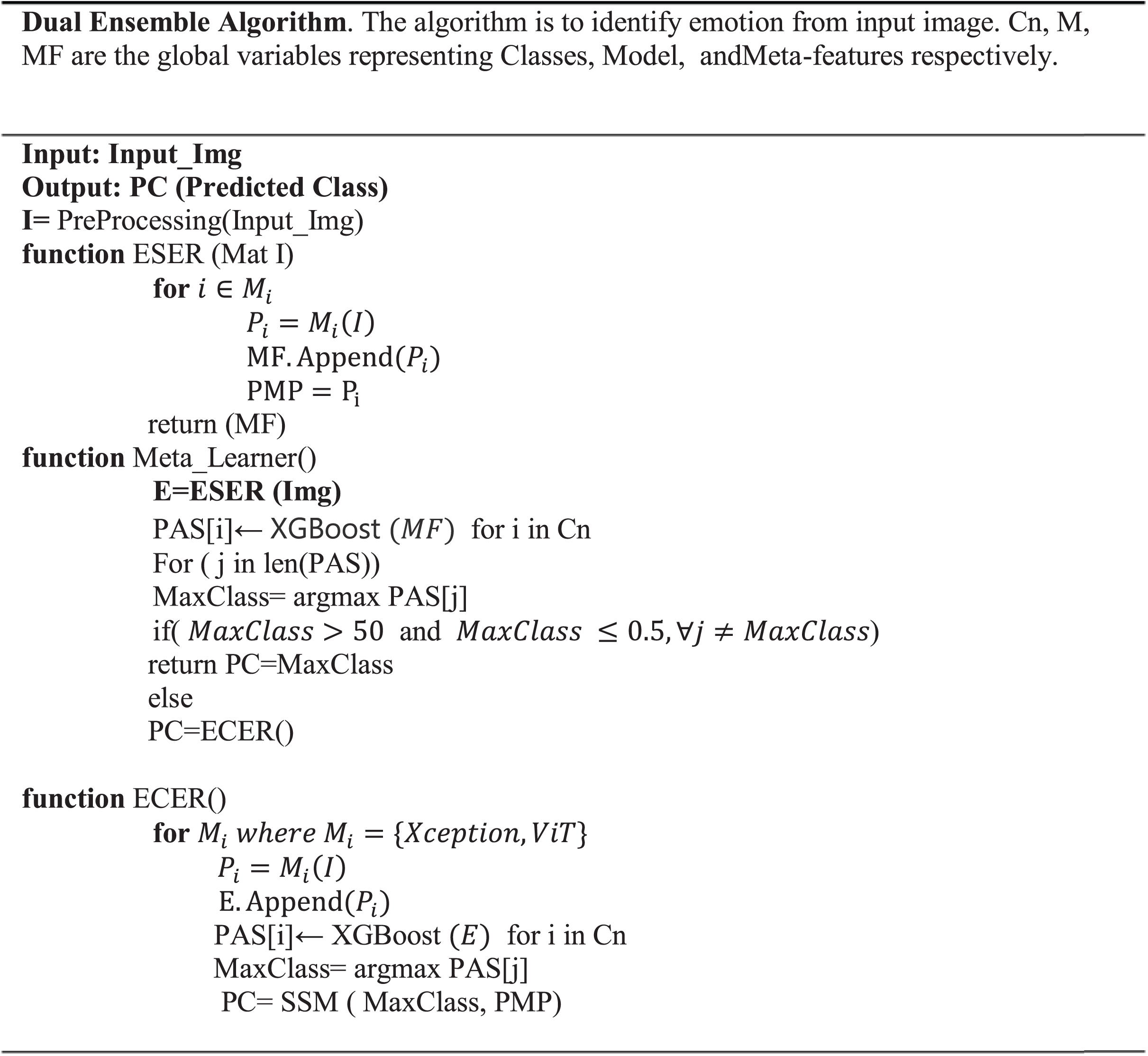
(6) where and for represents the standard happiness and standard sadness scores, respectively as shown in Table 1. To enhance the reliability of blended emotion classification, a SSM has been incorporated. Its operation is presented formally in Algorithm 1. The module accepts emotion-specific confidence values—primarily happiness and sadness scores—from the first ensemble stage. These values are then adjusted using pre-defined statistical weights and combined with predictions from the second ensemble using Eq. (6). Based on the computed net score (NS), the final emotional state is inferred. The entire procedure has been designed to provide additional support in cases of emotional ambiguity.
| Facial expression (Mixed emotion) | Happiness (%) | Sadness (%) |
|---|---|---|
| Bittersweet smile | 60% | 40% |
| Nostalgic look | 50% | 50% |
| Melancholic grin | 70% | 30% |
| Grateful sob | 65% | 35% |
| Regretful smile | 40% | 60% |
| Hopeful despair | 45% | 55% |
| Contented sadness | 55% | 45% |
| Joyful tears | 75% | 25% |
The algorithm of the framework is shown in Algorithm 1.
Base models
In the first phase (ESER), DenseNet169, VGG16, and ResNet50 are used as base models, while in the second phase (ECER), Xception and ViT are utilized. The selection of base models was made based on their proven effectiveness in image-based tasks and complementary architectural characteristics. DenseNet169 was chosen for its dense connectivity and efficient gradient propagation; VGG16 for its simplicity and feature depth; ResNet50 for its residual mapping capabilities. In the ECER phase, Xception was employed due to its depthwise separable convolutions, which reduce parameters while maintaining performance, and ViT was selected for its strong contextual learning ability through self-attention. These models have consistently demonstrated competitive performance in visual recognition tasks and were found to offer diverse representational strengths. Details about the base models are presented in the following subsections.
DenseNet169
The densely connected convolutional networks (DenseNet) follows the CNN architecture to improve gradient propagation. Unlike the traditional models, each layer in the network is connected to every other layer in a feed-forward fashion. Every connected layer is fed to layer . If is the feature maps of layers, then input to layer is given as;
(7)
Transformation with batch normalization ( ), activation by RelLU ( ) and convolution ( ) is performed at each connected layer to get final layer output as;
(8) For K layers in a dense block, outputs of the preceding layers are fed cumulatively to get the output of the dense layer as,
(9) where represents the DenseNet transformation.
The feature map in dense block as yielded by layer is represented as;
(10) where is the feature growth rate. A transition layer is utilized to perform down-sampling for shrinking the feature maps. Average pooling is preceded by convolution to efficiently reuse the features.
(11) After performing pooling globally, the SoftMax activation function with weight is applied to get the final classification.
(12)
VGG16
VGG16 is a CNN-based model containing 13 convolutional layers and three fully connected layers. To these layers, a filter is applied to capture details of an input image. Moreover, the feature map is reduced by recurrent stacks of convolutional layers trailed by the set of max-pool layers. If is the filter size where , and the spatial position in an input image with weight and bias , the convolution operation ( ) of VGG16 is given as,
(13) To take the maximum value from the window from the pooling window, the max-pooling (MP) operation of VGG16 is given as,
(14)
ResNet50
As the name implies, ResNet50 contains 50 layers (Huang et al., 2017). The model controls the vanishing gradient problem with residual learning. Similarly, the degradation of the neural networks is addressed by skip connections. Besides convolutional layers, batch normalization and ReLU activations, the model works on residual mappings. If is the input to a layer in the residual block with weight , output of the block after performing transformation is given as,
(15) For each input image , the following pre-residual operation is performed with Max Pooling (MP) to get stage 1st output- as,
(16) In the equation, represents batch normalization, which is applied to normalize the output and speed up the training process. If the input feature is , and , its mean and std. div. across the batch, then is given as;
(17)
Xception
The deep learning model Xception is effective in image classification tasks. Xception decouples the features of spatial and channel correlations. Batch normalization is preceded by standard convolution with ReLU as an activation function. The model promises to reduce the number of parameters without affecting performance. The depth-wise convolutions are stacked at the intermediate layer, whereas at the output layer, global average pooling is performed with a softmax activation function. Unlike traditional convolution, a feature map of height , width and channel is utilized to reduce computational cost. If is the filter size, x is the input tensor and the depthwise filter, the output at the position , in the feature map is given as,
(18) where is the filter weight of the convolution.
Vision transformer (ViT)
ViT is the transformer-based framework that extracts in-depth feature relationships by treating images as fixed-size patches of sequential tokens. Due to effective scaling, ViT outperforms other vision-based models like CNN. With ViT, a standard encoder transformer is applied to map inter-patch interactions. N number of patches of size is obtained for an input image of height and width as,
(19) The patches are flattened into a vector Which is used for the sequential embeddings- ,
(20) where and are the learnable weight and bias
Each sequence is then processed by multi-head self-attention ( ) layer and feed-forward ( ) network layer
(21) where and are the embedding-derived matrices and is the dimension of attention head.
Enhancing base model architecture
With each base model, the SE block is added to emphasize extracting informative features. The block is used to enhance the representational power of the neural networks. With the SE block, important features are adaptively weighted, thus allowing the base model to concentrate on the most relevant features. For an input tensor with channels of height and width , the block modulates the feature map via channel-wise scaling. Two main operations- squeezing and excitation are performed by the block. With squeezing, the spatial information is condensed into channels of a single value. For this purpose, global average pooling is performed to get vector. ,
(22) where being a global descriptor for channel ;
(23) With excitation, the importance of each channel is learned through the global optimizer . Two dense layers enact excitation. In between the two fully connected layers, non-linear activations is performed. The scaling factor used in the process is given as,
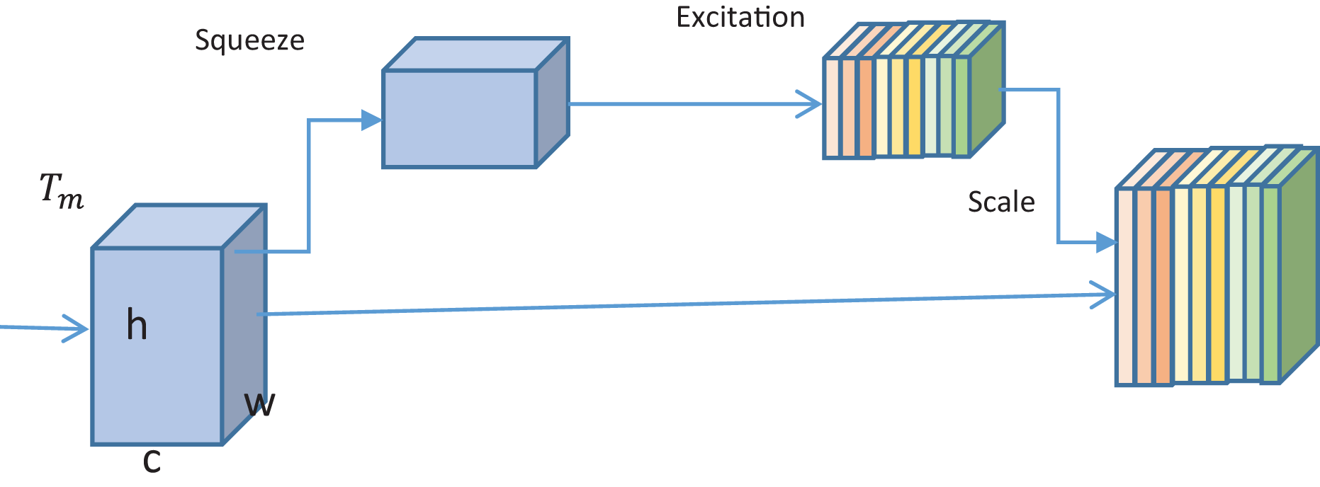
(24) where and are the weights of first and second fully connected layers. is the non-linear activation, while is the sigmoid function. As shown in Fig. 4, the output of dense layers is received as input by the SE block. In the block, squeezing and excitation are performed, followed by output scaling. The output of the SE block is fed to the following fully connected layers; see Fig. 4.
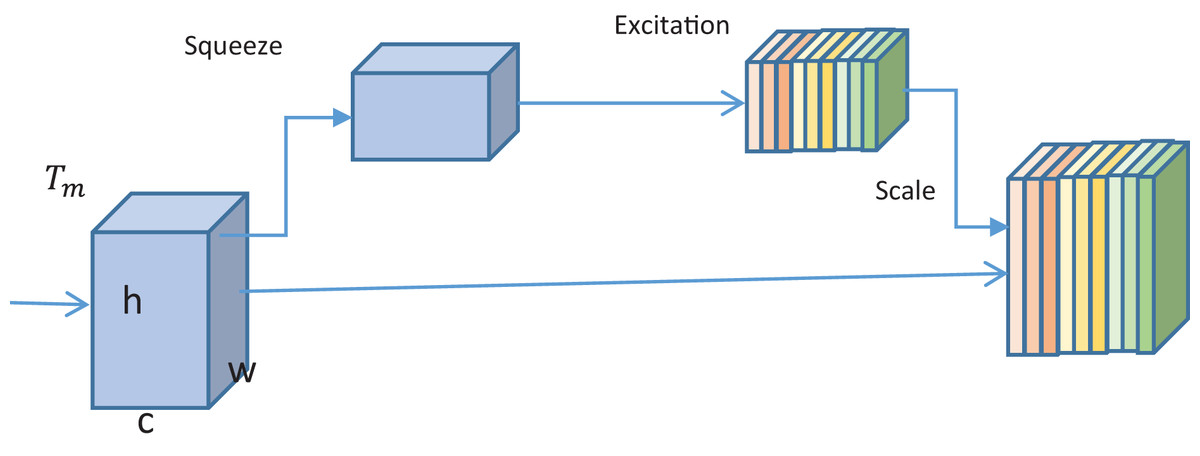
Figure 4: Illustration of the working of the SE block.
Meta model
In ensemble learning, XGBoost is used as a meta-model. Outputs of the base models are fed to the XGBoost classifier to extract the complex meta-features relationships and overcome overfitting. The meta-model guarantees promising image-based classification and robust decision-making. XGBoost has a scalable decision tree architecture where each tree at iteration, is fit to the residual errors (gradients) of the previous trees. XGBoost was selected as the meta-learner owing to its strong regularization capabilities, high training speed, and superior performance in classification tasks involving high-dimensional and correlated features. While simpler methods such as logistic regression or more complex models like neural attention layers could have been employed, XGBoost was preferred due to its balance between computational efficiency and predictive accuracy in ensemble learning scenarios. Its gradient-boosted framework has been observed to effectively exploit inter-model output relationships without overfitting. In dataset D, if X represents the feature vector and Y is the target label, such that and
, the objective function of XGBoost is given as,
(25) where is the loss function, is the predicted lable, is the regularization term, is for tree and T being the total number of trees. Regularization to avoid overfitting at tree ‘ ’ having tree leaves and weight is defined as follows.
(26) where and are the penalizing and regularization terms used in predicting label which is defined as,
(27) The loss function of XGBoost is given as,
(28) where is the log loss, and are the first and second-order gradients, respectively.
Evaluation
The models were trained with Adam (β1 = 0.9, β2 = 0.999), Initial Learning Rate: 0.001 with ReduceLROnPlateau scheduler, Batch Size: 64, Epochs: 100 for base models, 50 for meta-learner fine-tuning, Loss Function: Categorical Cross-Entropy, Validation Split: 15% and Early Stopping: Activated with patience of 10 epochs Hyperparameters were selected based on validation performance and empirical tuning across folds.
To analyze the performance of the dual ensemble architecture, the system is assessed by a total of 750 images of facial expressions containing 550 basic emotions and 200 blended emotions. Each base model captures spatial and hierarchical features differently, so their performance is observed distinctly beside the meta-model. Various metrics are observed, including accuracy, precision, recall, F1-score, and the area under the receiver operating characteristic curve (AUC-ROC). The evaluation outcomes testified that the ensemble method outperforms the individual models. The system’s performance is outstanding for basic emotions as an average 95% accuracy is achieved. However, for blended emotions, average accuracy of 88% is obtained. Details about the evaluation are presented in the following subsections.
Evaluation setup
A total of 3,750 images were taken from the Kaggle and IMED datasets for training, validation and testing. All the images were properly resized into fixed pixel sizes. Out of the total images, 70% were used for training, 15% for validation and 20% for testing. Before training, cross-validation was performed to avoid biases. In addition to cross-validation, several techniques were applied to prevent overfitting. Data augmentation methods such as horizontal flipping, random cropping, rotation, zooming, and brightness adjustments were consistently used across all training stages. Early stopping was also implemented during training to halt model updates if validation performance plateaued. Dropout layers were embedded within the classifier heads of certain base models to further enhance regularization. Stratified five-fold cross-validation was applied consistently across all models to maintain robustness and avoid bias. Furthermore, data augmentation techniques—including horizontal flipping, random rotations, zooming, and brightness variation—were uniformly performed during training. These steps were adopted to increase variability within the training set and reduce the likelihood of overfitting.
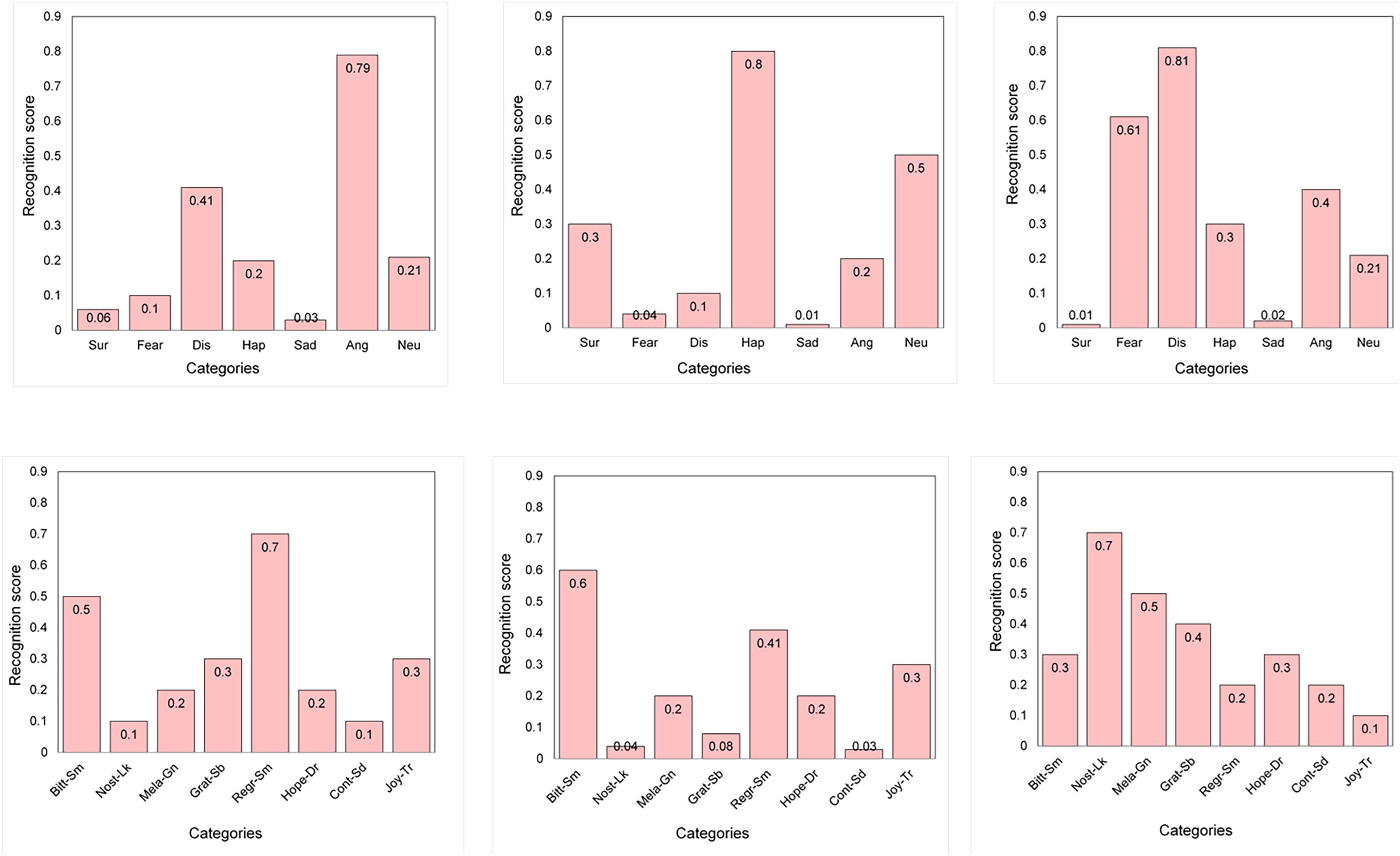
The results obtained during the two evaluations are locally stored in a separate text file for onward visualization and analysis. Following the establishment of the model architecture and training pipeline, experimental evaluation was conducted. The results and performance analysis of the ESER and ECER modules are discussed in the next section. An illustration of the recognition scores in the bar chart against the corresponding input images is presented in Fig. 5.
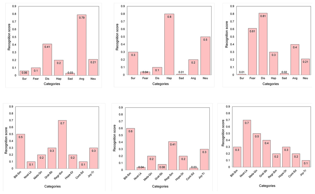
Figure 5: Illustration of the recognition scores in the bar chart.
Evaluation of ESER
The performance of the first ensemble framework- ESER, is assessed along with the individual performance of the base models. The average accuracy of base models of ESER is 89%, overtaken by the ensemble as 95% accuracy is obtained for XGBoost. The average F1-score of the base models is 0.85; with the ensemble, the score is raised to 0.95. In order to validate the improvements observed, paired t-tests were conducted between the ensemble predictions and those of each base model. For both ESER and ECER stages, p-values below 0.01 were recorded, indicating that the accuracy improvements achieved by the proposed ensembles are statistically significant and unlikely to have occurred by chance.
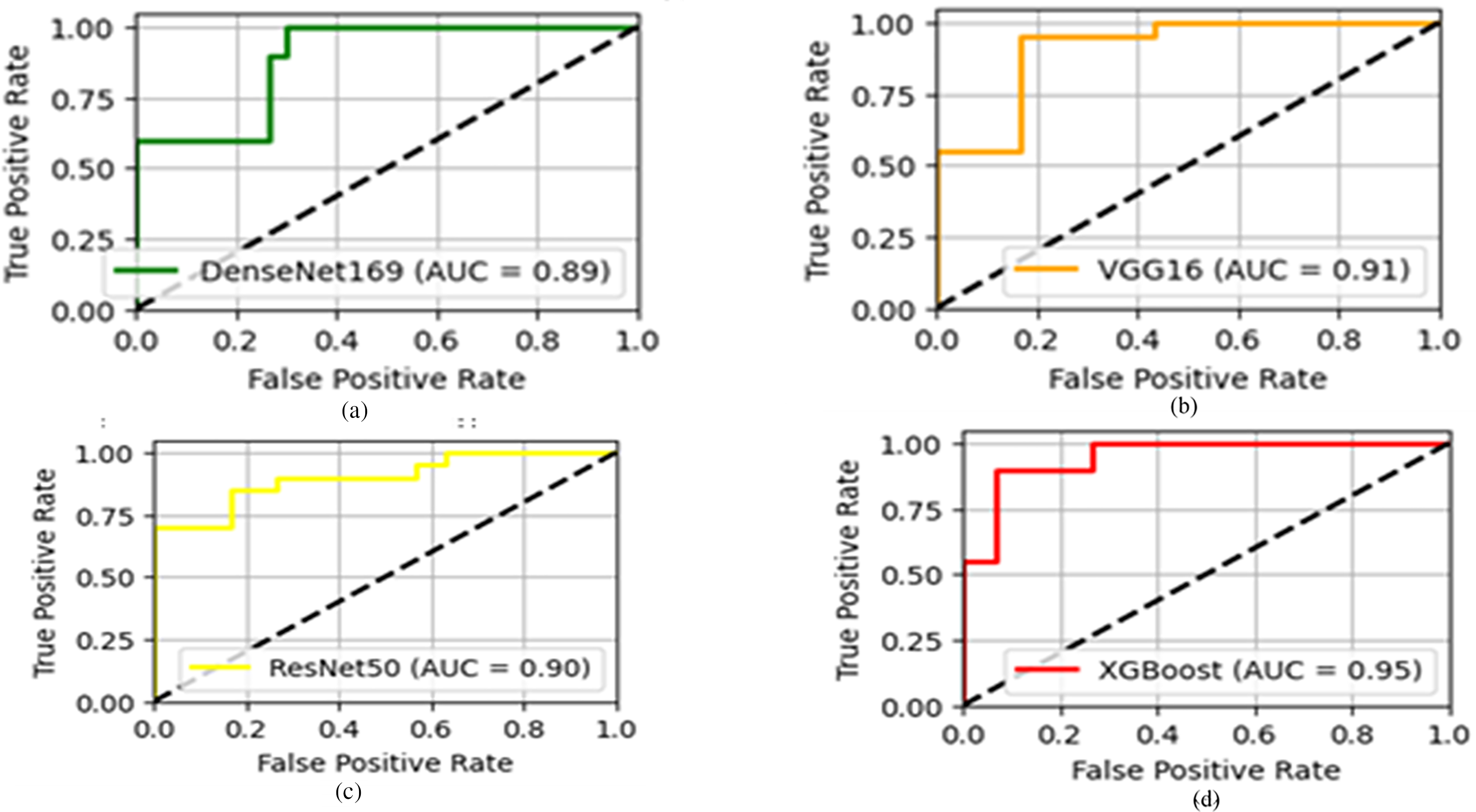
The Area Under Curve (AUC), precision, recall, accuracy, and F1-score of the base models and the ensemble method using XGBoost are shown in Table 2. The formulas used for computing precision (P), recall (R) and F1-score are given in Eqs. (28), (29) and (30), respectively.
| Model | AUC | Precision | Recall | Accuracy | F1-score |
|---|---|---|---|---|---|
| DenseNet169 | 0.89 | 0.85 | 0.87 | 0.88 | 0.86 |
| VGG16 | 0.91 | 0.91 | 0.89 | 0.91 | 0.89 |
| ResNet50 | 0.90 | 0.89 | 0.87 | 0.90 | 0.88 |
| XGBoost | 0.95 | 0.94 | 0.95 | 0.95 | 0.94 |
(29)
(30)
(31) If represents the number of correct classifications and the total number of predicted classes, accuracy A is given as,
(32) Similarly, if and are the coordinates of the points on the curve, then AUC is represented as,
(33) As clear from Fig. 6, the rapid climb of the meta-model at the top-left indicates the effective performance of the model. Moreover, the positive rate at the top-left of XGBoost with the highest accuracy of 95% suggests that the proposed ensemble method optimally recognized the emotions.
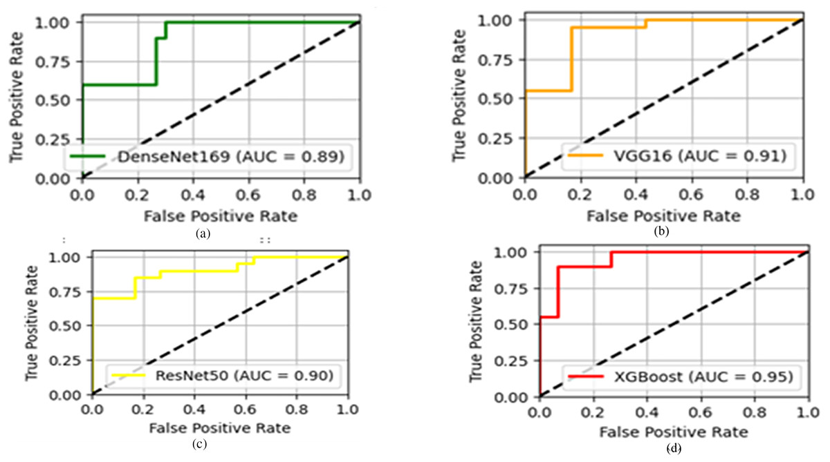
Figure 6: The AUCs of the (A) DenseNet (B) VGG16 (C) ResNet (D) and XGBoost model.
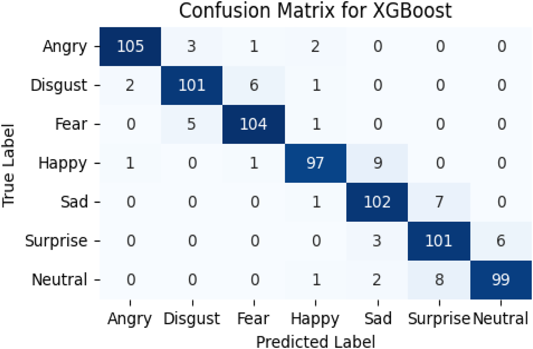
The confusion matrix of the recognition of basic emotions is shown in Fig. 7, while the statistics are in Table 3.
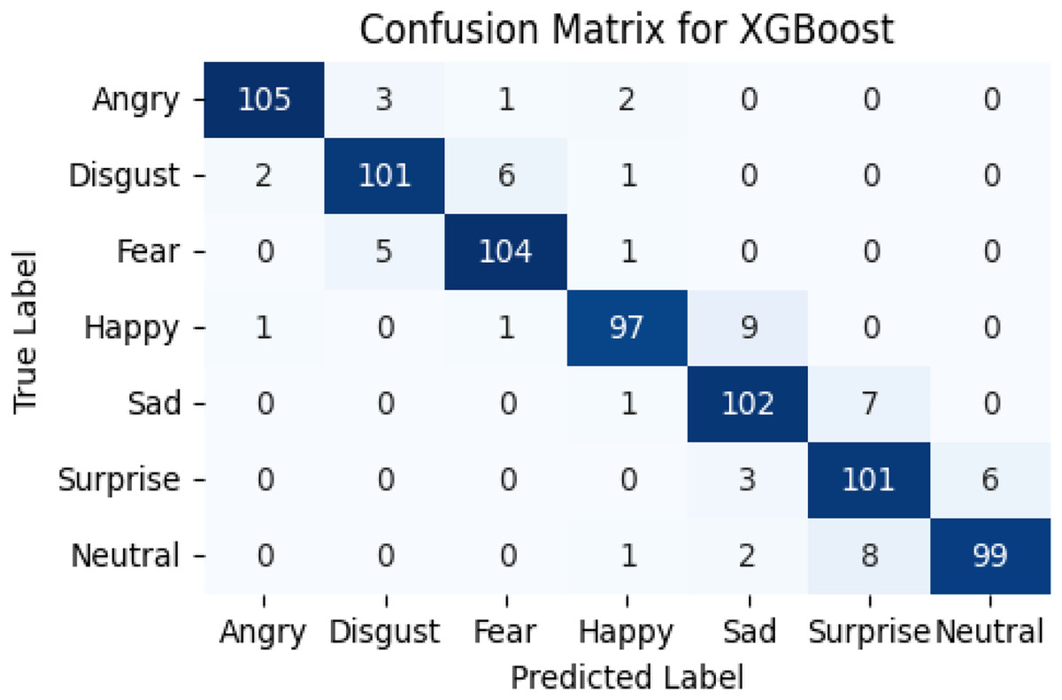
Figure 7: Confusion matrix of the meta-learner model.
| Model | Precision | Recall | F1-score |
|---|---|---|---|
| Angry | 0.98 | 0.95 | 0.96 |
| Disgust | 0.96 | 0.93 | 0.94 |
| Fear | 0.80 | 0.95 | 0.87 |
| Happy | 0.78 | 0.99 | 0.87 |
| Sad | 0.80 | 0.94 | 0.86 |
| Surprise | 0.80 | 0.94 | 0.86 |
| Neutral | 0.91 | 0.97 | 0.94 |
Evaluation of ECER
To mitigate class imbalance within the blended emotion dataset (IMED), oversampling techniques were applied during training. Specifically, minority emotion classes were augmented via data replication and perturbation-based synthesis to ensure balanced class representation. Additionally, class weights were adjusted during loss calculation in ECER to penalize misclassification of underrepresented categories more heavily. Blended emotion recognition is assessed separately by testing the system with 200 images of complex facial emotions. Though the individual performance of the ViT model is satisfactory, the meta-model outperforms the individual accuracies of the base models. Without the ensemble approach, the average accuracy is 70.45%, whereas an acceptable accuracy of 88.7% is achieved with the ensemble. The precision, recall and F1-score of the base models and XGboost are presented in Table 4.
| Xception | ViT | XGBoost | |||||||
|---|---|---|---|---|---|---|---|---|---|
| Model | Precision | Recall | F1-score | Precision | Recall | F1-score | Precision | Recall | F1-score |
| Bittersweet smile | 0.58 | 0.7 | 0.64 | 0.76 | 0.72 | 0.74 | 0.74 | 0.65 | 0.69 |
| Nostalgic look | 0.7 | 0.75 | 0.72 | 0.75 | 0.68 | 0.71 | 0.87 | 0.97 | 0.91 |
| Melancholic grin | 0.53 | 0.4 | 0.46 | 0.63 | 0.68 | 0.65 | 0.72 | 0.9 | 0.8 |
| Grateful sob | 0.69 | 0.72 | 0.71 | 0.71 | 0.72 | 0.72 | 0.92 | 0.82 | 0.87 |
| Regretful smile | 0.89 | 0.8 | 0.84 | 0.84 | 0.8 | 0.82 | 0.95 | 0.9 | 0.92 |
| Hopeful despair | 0.67 | 0.75 | 0.71 | 0.67 | 0.75 | 0.71 | 0.95 | 0.93 | 0.94 |
| Contented sadness | 0.68 | 0.68 | 0.68 | 0.64 | 0.68 | 0.66 | 0.95 | 0.97 | 0.96 |
| Joyful tears | 0.74 | 0.72 | 0.73 | 0.72 | 0.72 | 0.72 | 1.0 | 0.95 | 0.97 |
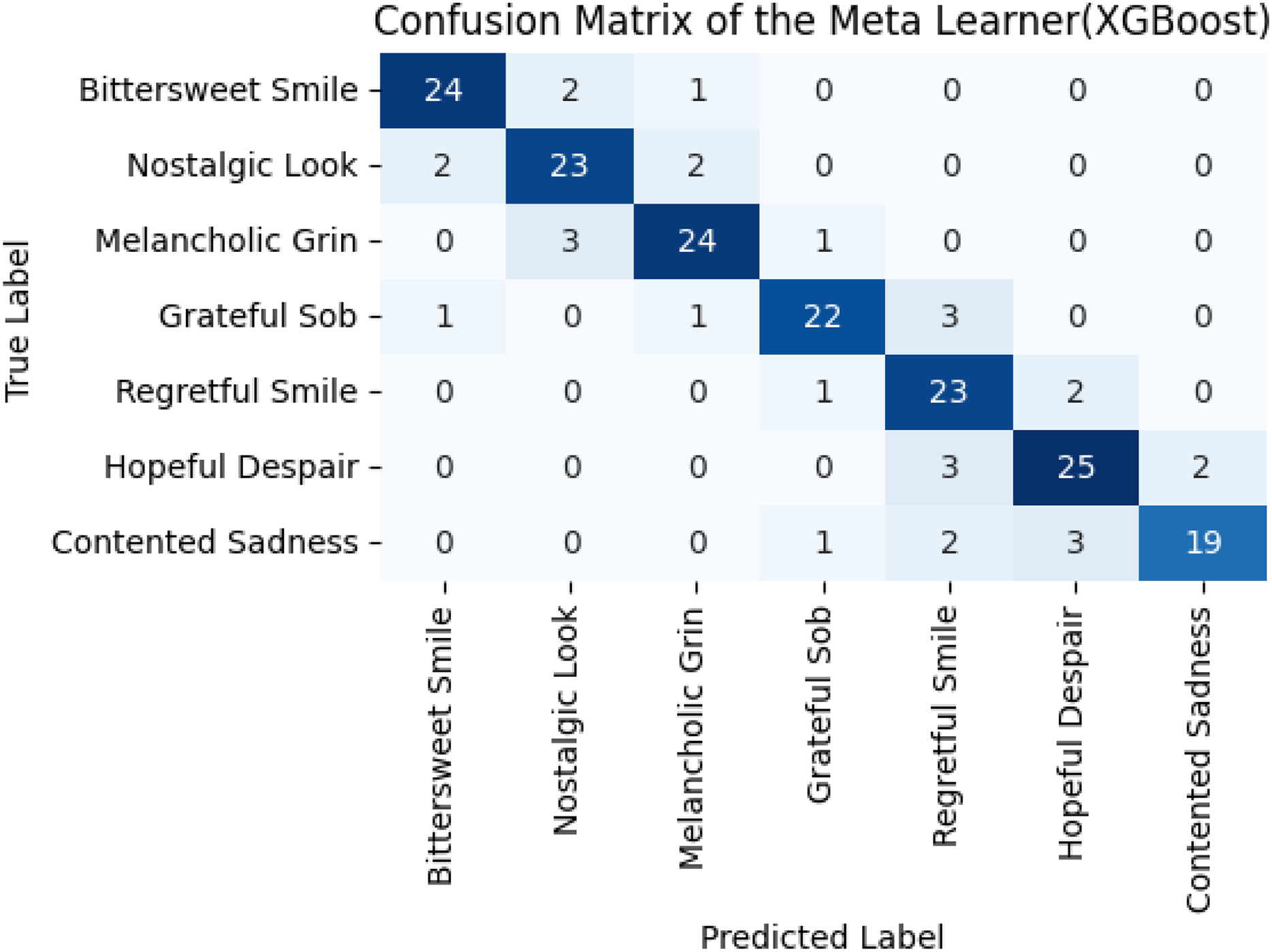
The reported average F1-score of the base models is 68% and 71%. However, a better F1-score (88%) was obtained for the ensemble. In addition to accuracy, other performance indicators such as F1-score, precision, recall, and ROC-AUC have been evaluated and presented in Tables S2A and S4A. These metrics were calculated to provide a more comprehensive understanding of the model’s classification behavior across all emotion categories. This implies that the ECER model effectively captures complex patterns and significantly lowers the chances of false negativity, as shown in Fig. 8.
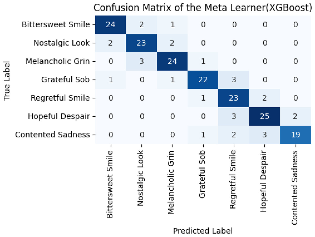
Figure 8: Confusion matrix of meta learners.
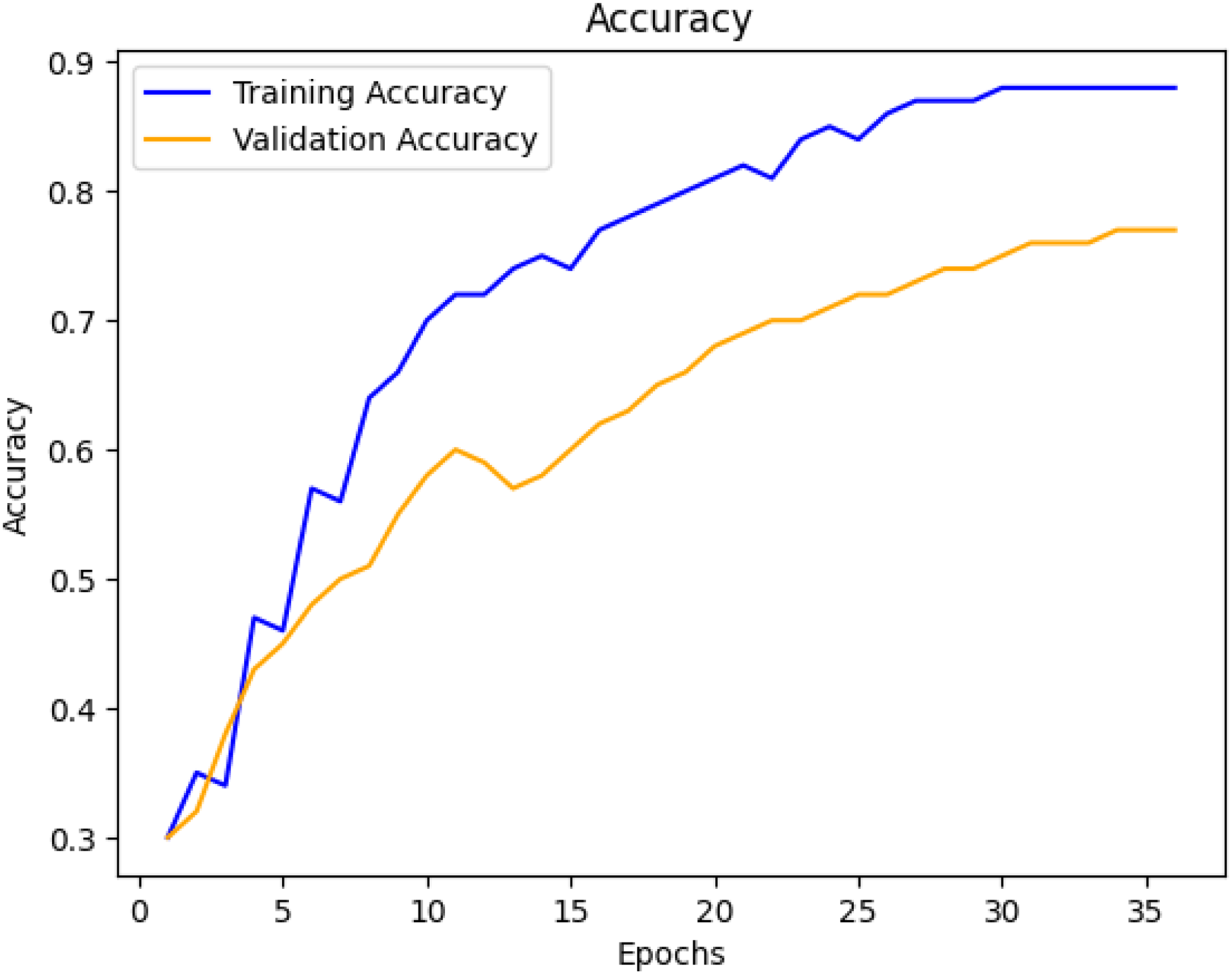
From the first few epochs, it can be assumed that the model’s accuracy improves as the number of epochs is increased, see Fig. 9.
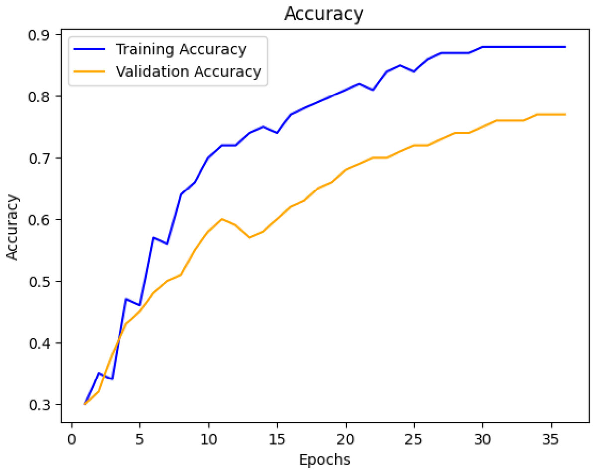
Figure 9: Model accuracy improvement.
Pruning approach assessment
Though the performance of the ensemble model is superior to the base model in terms of accuracy, the aggregation performed by XGBoost adheres to additional computational cost. To reduce computational complexity, the pruning approach is assessed to analyze its effect regarding accuracy and computational cost. The approach intends to exclude the least significant base models during inferencing stage without affecting the performance as a whole. The two least significant models- DensNet from the ESER and Xception from the ECER, were excluded from the list of base models. With this, the accuracies obtained for ESER and ECER are 87% and 83%, respectively. This shows that about 21% of the computational time can be minimized at the cost of about a 7.05% reduction in the accuracies. Results of the ensemble obtained after the pruning approach are presented in Table 5.
| Class | Precision | Recall | F1-score | Class | Precision | Recall | F1-score |
|---|---|---|---|---|---|---|---|
| Angry | 0.92 | 0.89 | 0.90 | BittSweet smile | 0.70 | 0.60 | 0.64 |
| Disgust | 0.89 | 0.86 | 0.87 | Nostalgic look | 0.85 | 0.92 | 0.88 |
| Fear | 0.75 | 0.86 | 0.80 | Melancholic grin | 0.68 | 0.85 | 0.75 |
| Happy | 0.70 | 0.88 | 0.78 | Grateful sob | 0.88 | 0.75 | 0.82 |
| Sad | 0.76 | 0.85 | 0.80 | Regretful smile | 0.90 | 0.85 | 0.87 |
| Surprise | 0.78 | 0.88 | 0.83 | Hopeful despair | 0.91 | 0.88 | 0.89 |
| Neutral | 0.85 | 0.90 | 0.87 | Contented sadness | 0.92 | 0.93 | 0.92 |
Discussion
As emotions are the common way to exhibit feelings, emotion recognition is a growing interest in human-computer interaction (Londhe & Pawar, 2012). The emerging ML-based technology for image classification can be rightly exploited for emotion recognition. With cutting-edge deep learning models, emotions can be detected precisely and aptly with no human involvement. Various systems have been proposed so far. However, no single model is strong enough to detect the emotions optimally. With ensemble methods, the strength of multiple models can be combined to improve classification. Though complex features are efficiently traced with a simple ensemble approach, the method suffers from various challenges like overfitting and generalization. To present a robust framework, this research proposes a dual ensemble framework for simple and blended emotion recognition. In the first ensemble (ESER), the classification of the seven universal emotions is performed. The eight blended emotions are identified in the second ensemble (ECER). At either level, a hybrid approach is followed to combine the strengths of the base models. Images of the dataset are properly preprocessed, where pixel normalization and resizing are performed before training and testing. Moreover, image augmentation was also performed to reduce the chances of overfitting by increasing variability. For effective training, the SE block is exploited to give higher weight to important features. The proposed method is evaluated to check how the ensemble improve classification. The average of individual accuracies of based models is 89% which is outperformed in the ensemble as 95% accuracy is achieved. Similarly, in the second level, the average accuracy of base models (71.45%) is surpassed by the ensemble approach and a promising 88.7% accuracy is achieved. The notable precision, recall and F1-score also highlights strength of the ensemble approach. As computational cost is an issue with ensemble method, the pruning approach is utilized to assess impact of pruning on accuracy. The least significant base models-DensNet and Xception were excluded in the pruning. Reports of the evaluations show that 21% of the computational cost can be avoided at the cost of 7.05% of the accuracy. This show effortless alteration in the framework for scenarios where computational cost is more crucial.
Conclusion and limitations
This research introduces a dual-ensemble deep learning framework for facial emotion recognition, addressing both primary and complex blended emotions. By integrating state-of-the-art models such as DenseNet169, VGG16, ResNet50, Xception, and ViT along with SE blocks, the approach effectively captures intricate facial expressions. The experimental results demonstrate that the framework achieves 95% accuracy for primary emotions and 88% accuracy for blended emotions, outperforming traditional unimodal methods. These findings highlight the potential of ensemble deep learning in enhancing human-computer interaction, psychological analysis, and affective computing applications. The proposed dual-ensemble architecture has been designed to offer generalizability across diverse facial expression datasets. Its two-stage learning strategy allows it to adapt to both well-defined and ambiguous emotional patterns. Moreover, by incorporating multiple base models and a meta-learning strategy, the framework is expected to retain performance robustness even when applied to unseen emotional combinations or data distributions from culturally different sources. The following are the main limitations we faced.
Future work
For the last decade or so, recognition of emotion from facial expression is becoming a rich research area for the scientific community. Unlike the traditional statistical approaches, the cutting edge deep learning models are effective in detecting and classifying emotions. However, as no such single model can optimally perform classification, ensemble approach is the right alternative to have the strengths of multiple state-of-the-art models. With this research work, a novel dual ensemble framework is introduced for the classification of typical and blended emotions. In the first ensemble model, results of the three base models are fed to the meta-learner whereas in the second level of ensemble two standard base models are utilized besides the aiding statistics. The inbuilt weakness of any single model is compensated and improved generalization is guaranteed. Results of the evaluation support effectiveness of the proposed method as average accuracy of 95% and 88.7% are achieved for the common and blended emotions. Though, with the pruning approach, computational cost is reduced, however explicit selection of the models is required to retain the accuracy. We are determined to enhance the model in future such that the least significant based models may be excluded automatically.