
Mesocarnivore landscape use along a gradient of urban, rural, and forest cover
- Published
- Accepted
- Received
- Academic Editor
- Jennifer Vonk
- Subject Areas
- Animal Behavior, Ecology, Zoology
- Keywords
- Bobcat (Lynx rufus), Coyote (Canis latrans), Gray fox (Urocyon cinereoargenteus), Raccoon (Procyon lotor), Striped skunk (Mephitis mephitis), Virgina opossums (Didelphis virginiana), Human disturbance, Activity, Mammalian carnivores, Landscape use
- Copyright
- © 2021 Rodriguez
- Licence
- This is an open access article, free of all copyright, made available under the Creative Commons Public Domain Dedication. This work may be freely reproduced, distributed, transmitted, modified, built upon, or otherwise used by anyone for any lawful purpose.
- Cite this article
- 2021. Mesocarnivore landscape use along a gradient of urban, rural, and forest cover. PeerJ 9:e11083 https://doi.org/10.7717/peerj.11083
Abstract
Mesocarnivores fill a vital role in ecosystems through effects on community health and structure. Anthropogenic-altered landscapes can benefit some species and adversely affect others. For some carnivores, prey availability increases with urbanization, but landscape use can be complicated by interactions among carnivores as well as differing human tolerance of some species. We used camera traps to survey along a gradient of urban, rural, and forest cover to quantify how carnivore landscape use varies among guild members and determine if a species was a human exploiter, adapter, or avoider. Our study was conducted in and around Corvallis, Oregon from April 2018 to February 2019 (11,914 trap nights) using 47 camera trap locations on a gradient from urban to rural. Our focal species were bobcat (Lynx rufus), coyote (Canis latrans), gray fox (Urocyon cinereoargenteus), opossum (Didelphis virginiana), raccoon (Procyon lotor), and striped skunk (Mephitis mephitis). Raccoon and opossum were human exploiters with low use of forest cover and positive association with urban and rural developed areas likely due to human-derived resources as well as some refugia from larger predators. Coyote and gray fox were human adapters with high use of natural habitats while the effects of urbanization ranged from weak to indiscernible. Bobcat and striped skunk appeared to be human avoiders with negative relationship with urban cover and higher landscape use of forest cover. We conducted a diel temporal activity analysis and found mostly nocturnal activity within the guild, but more diurnal activity by larger-bodied predators compared to the smaller species. Although these species coexist as a community in human-dominated landscapes throughout much of North America, the effects of urbanization were not equal across species. Our results, especially for gray fox and striped skunk, are counter to research in other regions, suggesting that mesopredator use of urbanized landscapes can vary depending on the environmental conditions of the study area and management actions are likely to be most effective when decisions are based on locally derived data.
Introduction
Habitat loss and fragmentation is one of the greatest threats to global biodiversity (Butchart et al., 2010; Seto, Guneralp & Hutyra, 2012). Urbanization and agricultural development are among the chief drivers of this phenomenon (Imhoff et al., 2004; Aronson et al., 2014), but a suite of human commensal species also benefit from anthropogenic landscapes (Baker & Harris, 2007; Soulsbury & White, 2016). This dichotomy is particularly true for mammalian carnivores, some of which are frequently extirpated while others reach their highest population densities in anthropogenic landscapes. Many mammalian carnivores benefit either from human-derived resources or release from predation in anthropogenic landscapes (Pickett et al., 2001; Prange, Gehrt & Wiggers, 2003; Gaston et al., 2005). The variable species response to human disturbance can complicate our understanding of community structure and landscape use of the urban-rural-forest matrix (Lesmeister et al., 2015; Moss, Alldredge & Pauli, 2016).
Species most susceptible to anthropogenic disturbance include those with large home ranges, low population densities, or low fecundity (Pimm et al., 2014). Apex predators, which frequently share these traits, have declined globally in fragmented and urbanized systems (Crooks & Soulé, 1999; Hollings et al., 2016) while many mesopredators with faster life histories, smaller home ranges, and higher fecundities have increased their distribution and abundance (Prugh et al., 2009; Santini et al., 2019). The ability of species to persist in anthropogenic environments is also a product of human attitudes that lead to the persecution of species, such as apex predators, that are thought to be dangerous or damaging to human interests (Kansky & Knight, 2014).
The local extirpation of apex predators can release herbivorous prey species and mesopredators (Ritchie & Johnson, 2009; Prugh et al., 2009). Although mesopredators can benefit from anthropogenic subsidies and predation release (Pickett et al., 2001; Prange, Gehrt & Wiggers, 2003; Gaston et al., 2005), they incur substantial risk in human-dominated landscapes (Woods, Mcdonald & Harris, 2003; Baker et al., 2004; Blanchoud, Farrugia & Mouchel, 2004). Risks in urban landscapes include increased vehicle traffic, lethal removals, and domesticated pets (Lowry, Lill & Wong, 2013; Soulsbury & White, 2016). Animals living within urban environments may consequently alter daily activity patterns compared to their rural or forested counterparts due to human activity during diurnal hours (Grinder & Krausman, 2001; George & Crooks, 2006). Individual species within diverse carnivore communities, such as bobcat (Lynx rufus), coyote (Canis latrans), gray fox (Urocyon cinereoargenteus), opossum (Didelphis virginiana), raccoon (Procyon lotor), and striped skunk (Mephitis mephitis), may partition time to maximize resource gain and reduce energy consumption by avoiding human areas during daylight hours (Schuette et al., 2013; Wang, Allen & Wilmers, 2015).
Here we combined camera traps across a landscape gradient of urban, rural, and forested land cover with occupancy models to quantify effects of the multi-scaled landscape features on landscape use by mesopredators, including bobcat, coyote, gray fox, opossum, raccoon, and striped skunk, while accounting for imperfect detection (Lindstedt, Miller & Buskirk, 1986; Crooks, 2002). Within this guild of mesopredators, we expected some species would be human commensals while others would have less affinity towards human development. We expected to classify species as human avoiders, human adapters, or human exploiters (Blair, 1996; Riggio et al., 2018). Species that were positively associated with natural habitats and negatively associated with human developments were classified as human avoiders. Species that were negatively associated with natural habitats and positively associated with urbanization were classified as human exploiters. Species that did not show strong preference for either natural or human habitats were classified as human adapters. We assessed the response of each species to land cover type across three spatial scales (100 m, 500 m, and 1000 m) to determine the most important scale of response. Spatial scale is important when predicting species use (e.g., Gompper et al., 2016), and we expected that smaller species would respond to differences in cover types at a finer scale (Jetz et al., 2004).
Based on previous research, we predicted that the larger-bodied mesopredators (coyote and particularly bobcat) would be human avoiders that were negatively associated with anthropogenic disturbance (Atwood, Weeks & Gehring, 2004; Clare, Anderson & Macfarland, 2015; Lesmeister et al., 2015; Flores-Morales et al., 2019). In many regions raccoon and opossum have been found associated with urban habitats that provide human-subsidized resources and reduced risk from natural predators, so we expected them to be human exploiters in our study area (Prange, Gehrt & Wiggers, 2003; Bateman & Fleming, 2012). We predicted that gray fox and striped skunk would be human adapters with limited affinity for, or avoidance, of anthropogenic landscapes. Striped skunks are known to use human structures as denning sites (Theimer et al., 2017) and are commonly associated with rural human settlements (Lesmeister et al., 2015). Gray fox is commonly described as a species that associates with human development (Riley, 2006; Lesmeister et al., 2015), but that association can vary greatly between study areas and may relate more to site specific factors such as interference competition for prey or the prevalence of free-ranging dogs (Morin et al., 2018). We anticipated modest responses to forests, grasslands, and wetlands among species because all are capable of exploiting a variety of vegetation types, with the exception of raccoon, which we expected would be substantially associated with water cover (Henner et al., 2004).
Materials and Methods
Subjects
We classified our six target species (bobcat, coyote, gray fox, opossum, raccoon, and striped skunk) into three categories of human relationship (exploiter, adapter, and avoider) based on their occupancy use related to landscape features. From Blair (1996), exploiters will reach greater densities in sites with urban development and avoiders will be sensitive to features such as housing development and roads while preferring less disturbed natural areas like forests and grassland. Adapters will not fit neatly into the previous two classifications, but would be expected to benefit from additional human supplied resources like shelter and food (Blair, 1996; Riggio et al., 2018). We classified species as human adapters if there was no indication of a strong relationship with urban features, positive or negative. We expected these species to perhaps show weak relationships with both natural and anthropogenic landscape features. Landscape features we considered associated with human development were urban cover, distance to structure, and paved and unpaved roads. Forest cover, grassland cover, water cover, and distance to water were considered natural features when classifying our species.
Study area
We conducted a camera trap survey across urban, rural, and forested cover types in and around Corvallis, Oregon, USA (Fig. 1). We considered urban camera stations those that were within the city limits of Corvallis. Camera traps defined as rural were placed at sites outside city limits but remained on lands with human dwellings with the appropriate permission from landowners. The forest cover type was restricted to the MacDonald-Dunn Research Forest that bordered Corvallis to the northwest and contained no human dwellings.
According to the U.S. Census Bureau (2018), Corvallis had a population of 58,641 and covers 54.67 km2. The population density was 1,547.2/km2, with an average housing unit density of 665.4/km2 (US Census Bureau, 2018). Corvallis, and the rest of the Willamette Valley in Oregon, is located in the dry-summer temperate climate zone, or cool-summer Mediterranean (Kottek et al., 2006). The climate was characterized by year-round mild temperatures with warm, dry summers and cool, wet winters. Average yearly precipitation in Corvallis was 110.9 cm and an average high temperature of 63.4°F (17.4 °C) and an average low temperature of 41.9°F (5.5 °C). The average high and low temperatures in January were 47.0°F (8.3 °C) and 33.6°F (0.9 °C) respectively, and average precipitation of 16.4 cm (US Climate Data, 1981-2010). The average high and low temperatures in July were 81.2°F (27.3 °C) and 51.8°F (11.0 °C) respectively, and average precipitation of 1.4 cm (US Climate Data, 1981-2010).
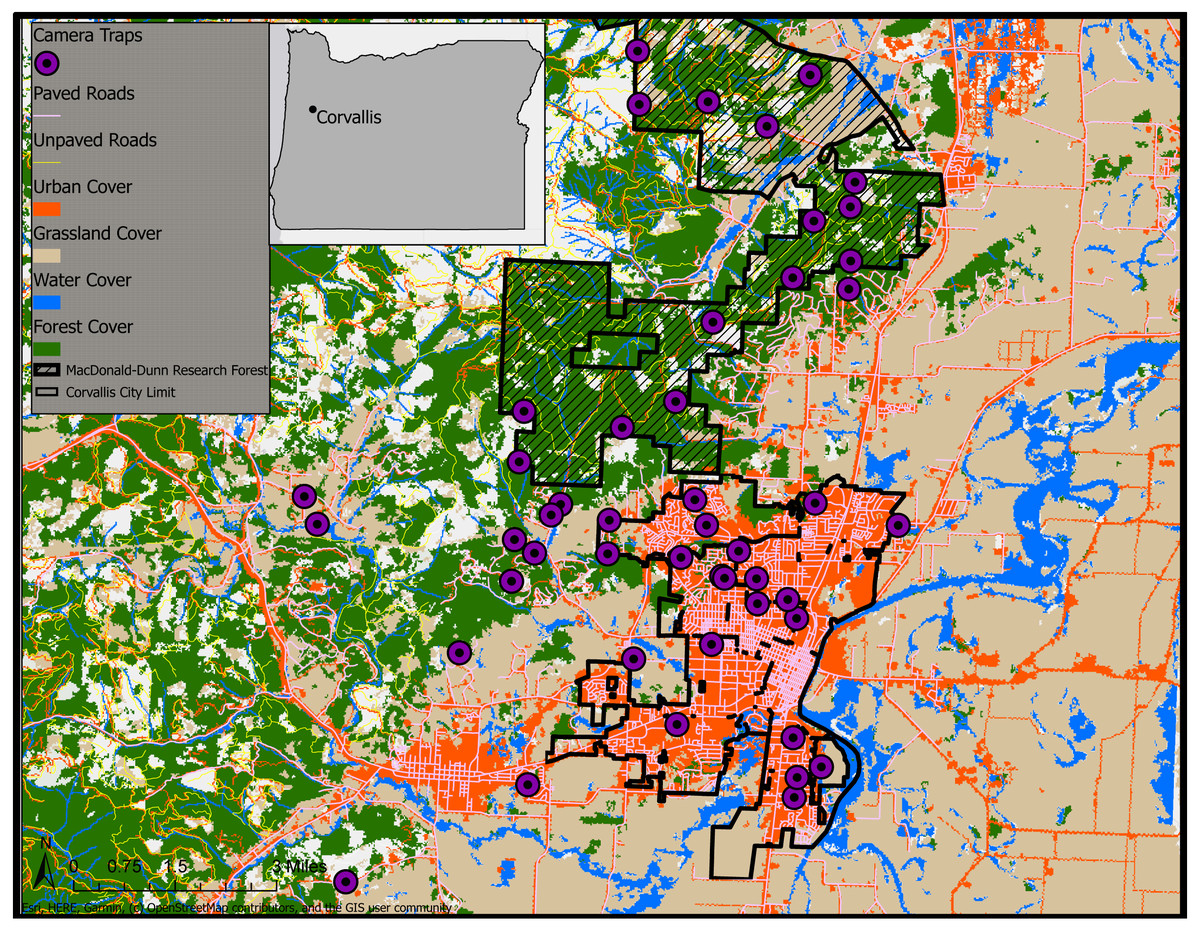
Figure 1: Land cover classifications (NLCD 2011) and camera trap survey locations in Corvallis, Benton County, Oregon, USA, April 2018–February 2019.
Map data ©2019 OpenStreetMap contributors.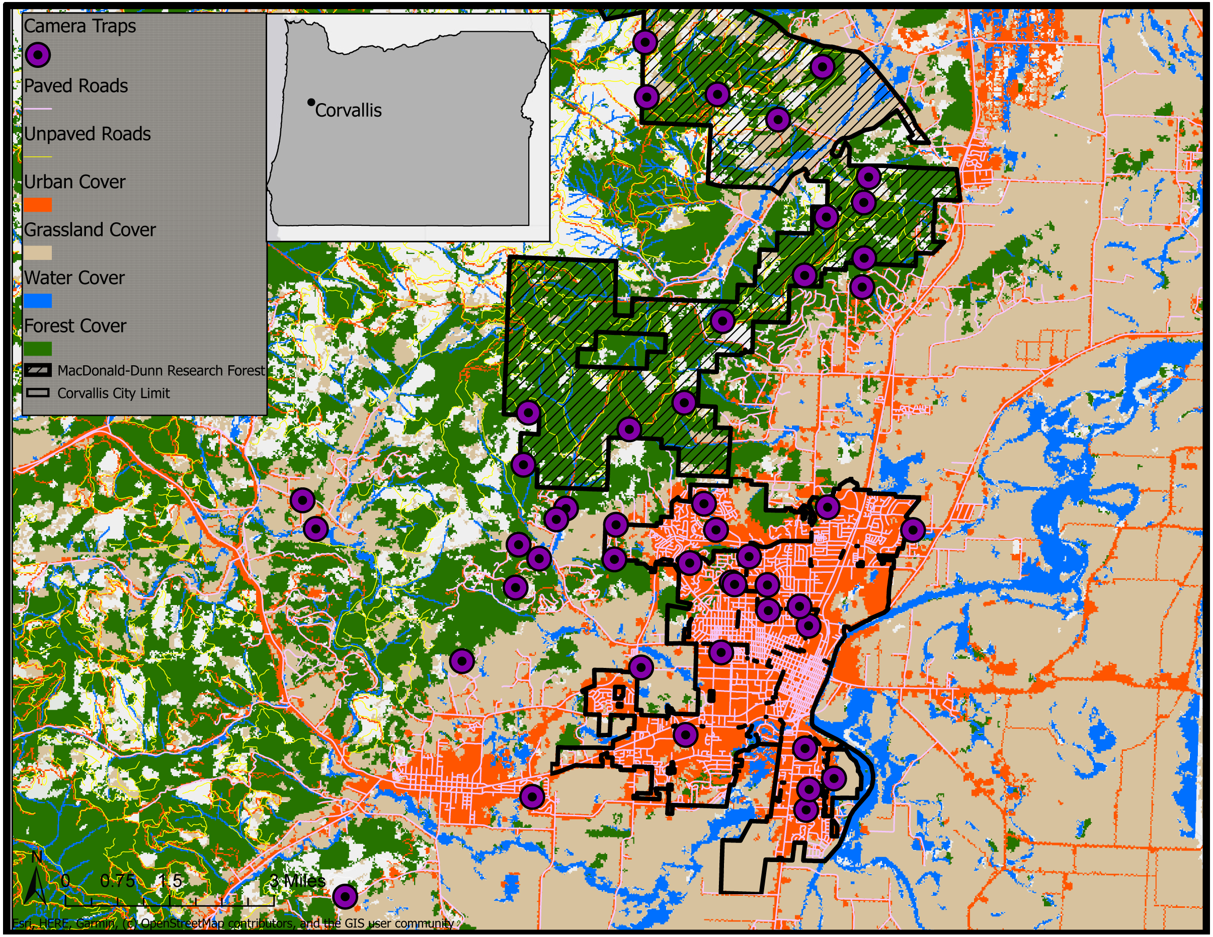
The McDonald-Dunn Research Forest was managed by Oregon State University and open to public recreation. The forest was over 4450 ha and rested in the eastern foothills of Oregon’s coastal mountain range, extending into the western Willamette Valley (Edson & Wing, 2011). Historically, much of the lowland MacDonald-Dunn Research Forest was dominated by oak savannas, but due to disturbance and other environmental conditions the forest was dominated by an overstory of Douglas fir (Pseudotsuga menziesii) (Fletcher et al., 2005). Other common native species include big-leaf maple (Acer macrophyllum), vine maple (A. circinatum), Oregon grape (Mahonia aquifolium), and western sword fern (Polystichum munitum). The McDonald-Dunn Research Forest was subject to four different forest management types (even-aged, two-storied, uneven-aged, and reserved old-growth stands) (OSU Research Forests). The forest was not open to public vehicle access but does receive over 175,000 recreation visits per year.
Site selection and data collection
We deployed 47 non-baited camera traps (Bushnell, Overland Park, KS, Trophy Cam HD) at urban, rural, and forest sites extending out from Corvallis, Oregon during April–June 2018. We revisited sites every four to six weeks to collect image data and service camera traps for a total of 41 weeks. We placed camera traps on private landowner properties as well as the MacDonald-Dunn Research Forest. We selected locations along the urban to rural gradient to sample as evenly as possible across the densest areas of Corvallis to the lesser populated rural dwellings surrounding the city. We attempted to select locations for camera traps that were no closer than 500 m to avoid redundancy in animal detections and land cover sampled. However, there were instances of camera trap locations that fell within this 500 m buffer due to our site selection process relying upon voluntary involvement from private landowners. Spacing of sampling sites was easier in the MacDonald-Dunn Research Forest since we were not restricted by property ownership and permissions from multiple landowners. Our goal for site selection was to get an even distribution of cameras between our three zones: urban, rural, and forest. We deployed 18 camera traps in urban areas, 14 in rural areas, and 15 in the MacDonald-Dunn Research Forest. A variety of cover types were selected for camera trap placements: mature forest, young forest, thinned stands, clear cuts, oak savannas, and riparian zones.
We placed camera traps at the bases of trees, fence posts, or other suitable structures approximately 50 cm off the ground. We set the cameras to record the time, date, temperature, and lunar phase of each image. We adapted our camera settings based on previous studies such as Wang, Allen & Wilmers (2015). We set the cameras to take three images in rapid succession for each detection event to improve the chances of species identification. A quiet period of one minute was set after a detection event to reduce duplicate detections of the same individual detection event and conserve battery life. We noted that previous findings from Ridout & Linkie (2009) found that a 30 min delay was a useful time delay in discerning detections of the same species, however our analysis did not rely significantly on individual activity patterns. We identified and tagged images by species and used those detections to generate weekly encounter histories for each species at each site so that one or more detections weekly was coded as “1” and no detections as “0”.
Survey and site variables
We summarized weekly temperature (TEMP) and precipitation (PRECIP) data that were collected from a nearby weather station (Corvallis, Oregon AgriMet Weather Station) to use in our detection probability models. We also used a binary factor to indicate that the camera was placed on an unpaved road (ONROAD; Table 1).
| Covariate | CODE | Description |
|---|---|---|
| precipitation | PRECIP | sum of weekly precipitation recorded from Corvallis weather station (AgriMet Station) |
| temperature | TEMP | average weekly temperature recorded from Corvallis weather station (AgriMet Station) |
| camera on road | ONROAD | whether or not a camera was placed on a road |
| distance to human structure | DTSTRUC | distance (m) to nearest human structure, measured with rangefinder if structure was visible; if not visible, measured with GIS |
| distance to surface water | DTWATER | distance (m) to nearest surface water measured with GIS |
| density of unpaved roads 100 m | USUMRD100 m | sum of unpaved road length in 100 m buffer around site |
| density of unpaved roads 500 m | USUMRD500 m | sum of unpaved road length in 500 m buffer around site |
| density of unpaved roads 1000 m | USUMRD1000 m | sum of unpaved road length in 1000 m buffer around site |
| density of paved roads 100 m | PSUMRD100 m | sum of paved road length in 100 m buffer around site |
| density of paved roads 500 m | PSUMRD500 m | sum of paved road length in 500 m buffer around site |
| density of paved roads 1000 m | PSUMRD1000 m | sum of paved road length in 1000 m buffer around site |
| forest cover 100 m | FC100 m | percent forest cover in a 100 m buffer around survey site measured with GIS |
| forest cover 500 m | FC500 m | percent forest cover in a 500 m buffer around survey site measured with GIS |
| forest cover 1000 m | FC1000 m | percent forest cover in a 1000 m buffer around survey site measured with GIS |
| urban cover 100 m | UC100 m | percent urban cover in a 100 m buffer around survey site measured with GIS |
| urban cover 500 m | UC500 m | percent urban cover in a 500 m buffer around survey site measured with GIS |
| urban cover 1000 m | UC1000 m | percent urban cover in a 1000 m buffer around survey site measured with GIS |
| grassland cover 100 m | GC100 m | percent grassland cover in a 100 m buffer around survey site measured with GIS |
| grassland cover 500 m | GC500 m | percent grassland cover in a 500 m buffer around survey site measured with GIS |
| grassland cover 1000 m | GC1000 m | percent grassland cover in a 1000 m buffer around survey site measured with GIS |
| water cover 100 m | WC100 m | percent water cover in a 100 m buffer around survey site measured with GIS |
| water cover 500 m | WC500 m | percent water cover in a 500 m buffer around survey site measured with GIS |
| water cover 1000 m | WC1000 m | percent water cover in a 1000 m buffer around survey site measured with GIS |
We used program ArcGIS (ESRI, Redlands, CA) to generate 100 m, 500 m, and 1000 m buffers around each camera trap site. Using the 2011 National Land Cover Data (Multi-Resolution Land Characteristics Consortium), we summarized forest (deciduous, evergreen, and mixed forest), urban development (open space, low intensity, medium intensity, high intensity), grassland (hay/pasture and cultivated crops), and water (streams, woody wetland, emergent herbaceous wetland, surface water) land cover classes. Within each buffer, we created spatial variables by calculating the proportion of land cover classes of forest (FC100M, FC500M, FC1000M), urban (UC100M, UC500M, UC1000M), grassland (GC100M, GC500M, GC1000M), and water (WC100M, WC500M, WC1000M). We used data from the Oregon Department of Transportation (Oregon Spatial Data Library) to calculate the summed length of unpaved roads (USUMRD100M, USUMRD500M, USUMRD1000M) and paved roads (PSUMRD100M, PSUMRD500M, PSUMRD1000M). We used data from the Oregon Water Resources Department (Oregon Spatial Data Library) to determine the distance to surface water (DTWATER) from each camera trap. If a human structure was visible from the camera site, we calculated the distance (DTSTRUC) using a rangefinder (Table 1). If no structure was immediately visible, we used aerial imagery in ArcGIS to measure distance.
Temporal activity analysis
The time and date of each image in our study was recorded. Images of the same species were not included in the temporal activity analysis if they were observed within 30 min of each other to reduce pseudoreplication (Ridout & Linkie, 2009; Lucherini et al., 2009; Wang, Allen & Wilmers, 2015). We reasoned that detections >30 min apart at unbaited cameras could be assumed independent events in activity analysis. Detection events with two or more individuals of the same species were counted as a single event. In the case of two different species in a single image, the event was recorded once for each species. We used the camtrapR 1.5.3 package (Niedballa et al., 2016) in RStudio 3.5.3 to create single-species diel activity kernel density estimation plots.
Occupancy modeling
We used Program Presence 2.12.17 and RPresence 2.12.17 (Mackenzie et al., 2002; Hines, 2006; MacKenzie, Nichols & Royle, 2018) in a two-stage approach to fit and rank our single-species single-season occupancy models (MacKenzie, Nichols & Royle, 2018). First, we modeled our survey level covariates (TEMP, PRECIP, and ONROAD) against a null (.) detection model to determine which covariate was most supported for detection probability (p) (Appendix A). We used the most supported model structure based on The Akaike information criterion (Akaike, 1974) for small sample sizes (AICc) values for detection probability in subsequent models that included covariates for occupancy (Ψ). We then fit univariate occupancy models and varied the value of the focal covariate based on three different buffers (100 m, 500 m, 1000 m). We carried forward the buffer scale with the most AICc weight for use in our multivariate models. We did not include covariates in the same multivariate model if their correlation coefficient had a magnitude >—.6—. In general, correlated covariates included covariates of the same cover type at different spatial scales. At most spatial scales, paved road density was negatively correlated with forest cover and positively correlated with urban cover. Unpaved road density was positively correlated with distance to structures. For each species, we compared the strength of multivariate models (including intercept only) and carried forward the models (and associated covariate beta coefficients) that collectively comprised >90% of model weight into our analysis (Table 2, Appendix B). We relied on model weight for final model selection rather than the ΔAICc ≤ 2 threshold because it has been found to be insufficient for within-stage model selection (Morin et al., 2020) and may exclude models with strong support.
Results
Our 47 cameras were operational for 11,914 trap nights over the 41-week study period yielding 23,988 images of 14 identified vertebrate species. Columbian black-tailed deer (Odocoileus hemionus columbianus) were the most commonly detected species (n = 5371) at 42 sites. Raccoon was the most commonly detected carnivore (n = 1964) at 29 sites. There were 1680 detections of opossum at 31 sites, 471 detections of gray fox at 19 sites, 415 detections of striped skunk at 18 sites, 171 detections of coyote at 13 sites, and 134 detections of bobcat at 20 sites. We detected cougar (Puma concolor) 30 times at eight sites. Black bear (Ursus americanus) was detected once at a single site.
| Modela | Δ AICcb | ωc | Kd | neg2lle | βf | seg | |
|---|---|---|---|---|---|---|---|
| Bobcat (Lynx rufus) | |||||||
| Ψ(UC100 m+GC100 m), p (ONROAD) | 0 | 0.3415 | 5 | 569.55 | Ψ(UC100 m) | −1.080 | 0.430 |
| Ψ(GC100 m) | 0.786 | 0.645 | |||||
| p(ONROAD) | 1.068 | 0.251 | |||||
| Ψ(UC100 m), p (ONROAD) | 0.23 | 0.3047 | 4 | 572.29 | Ψ(UC100 m) | −1.184 | 0.412 |
| p(ONROAD) | 1.053 | 0.247 | |||||
| Ψ(GC100 m+FC1000 m), p (ONROAD) | 2.21 | 0.1129 | 5 | 571.76 | Ψ(GC100 m) | 1.139 | 0.615 |
| Ψ(FC1000 m) | 0.811 | 0.359 | |||||
| p(ONROAD) | 1.049 | 0.247 | |||||
| Coyote (Canis latrans) | |||||||
| Ψ(USUMRD100 m+WC500 m), p (Precip) | 0 | 0.140 | 5 | 844.12 | Ψ(USUMRD100 m) | 0.785 | 0.374 |
| Ψ(WC500 m) | 0.729 | 0.394 | |||||
| p(Precip) | −0.541 | 0.116 | |||||
| Ψ(WC500 m+FC100 m), p (Precip) | 0.85 | 0.092 | 5 | 844.97 | Ψ(WC500 m) | 0.781 | 0.416 |
| Ψ(FC100 m) | 0.740 | 0.370 | |||||
| p(Precip) | −0.541 | 0.116 | |||||
| Ψ(USUMRD100 m+WC500 m+FC100 m), p (Precip) | 1.75 | 0.059 | 6 | 843.23 | Ψ(USUMRD100 m) | 0.554 | 0.437 |
| Ψ(WC500 m) | 0.832 | 0.423 | |||||
| Ψ(FC100 m) | 0.407 | 0.437 | |||||
| p(Precip) | −0.541 | 0.116 | |||||
| Gray Fox (Urocyon cinereoargenteus) | |||||||
| Ψ(GC1000 m), p (ONROAD) | 0 | 0.426 | 4 | 757.62 | Ψ(GC1000 m) | 1.192 | 0.419 |
| p(ONROAD) | −1.558 | 0.269 | |||||
| Ψ(GC1000 m+PSUMRD500 m), p (ONROAD) | 0.87 | 0.276 | 5 | 755.97 | Ψ(GC1000 m) | 1.087 | 0.420 |
| Ψ(PSUMRD500 m) | −0.470 | 0.380 | |||||
| p(ONROAD) | −1.566 | 0.271 | |||||
| Ψ(GC1000 m+UC500 m), p (ONROAD) | 2.5 | 0.122 | 5 | 757.61 | Ψ(GC1000 m) | 1.182 | 0.430 |
| Ψ(UC500 m) | −0.034 | 0.350 | |||||
| p(ONROAD) | −1.558 | 0.269 | |||||
| Opossum (Didelphis virginiana) | |||||||
| Ψ(DTSTRUC), p (Temp) | 0 | 0.1863 | 4 | 1459.36 | Ψ(DTSTRUC) | −1.777 | 0.660 |
| p(Temp) | 0.209 | 0.067 | |||||
| Ψ(DTSTRUC+UC100 m), p (Temp) | 0.015 | 0.1848 | 5 | 1456.86 | Ψ(DTSTRUC) | −1.204 | 0.617 |
| Ψ(UC100 m) | 0.804 | 0.571 | |||||
| p(Temp) | 0.209 | 0.067 | |||||
| Ψ(USUMRD500 m), p (Temp) | 0.467 | 0.1475 | 4 | 1459.83 | Ψ(USUMRD500 m) | −1.322 | 0.406 |
| p(Temp) | 0.209 | 0.067 | |||||
| Raccoon (Procyon lotor) | |||||||
| Ψ(rDTSTRUC), p (ONROAD) | 0 | 0.392 | 4 | 1414.47 | Ψ(DTSTRUC) | −1.573 | 0.633 |
| p(ONROAD) | −2.595 | 0.376 | |||||
| Ψ(DTSTRUC+PSUMRD100 m), p (ONROAD) | 2.05 | 0.1404 | 5 | 1414.02 | Ψ(DTSTRUC) | −1.318 | 0.688 |
| Ψ(PSUMRD100 m) | 0.311 | 0.469 | |||||
| p(ONROAD) | −2.581 | 0.374 | |||||
| Ψ(DTSTRUC+UC500 m), p (ONROAD) | 2.47 | 0.1139 | 5 | 1414.44 | Ψ(DTSTRUC) | −1.494 | 0.734 |
| Ψ(UC500 m) | 0.088 | 0.445 | |||||
| p(ONROAD) | −2.591 | 0.376 | |||||
| Skunk (Mephitis mephitis) | |||||||
| Ψ(FC500 m), p (ONROAD) | 0 | 0.3583 | 4 | 708.01 | Ψ(FC500 m) | 0.875 | 0.337 |
| p(ONROAD) | −0.674 | 0.222 | |||||
| Ψ(PSUMRD100 m), p (ONROAD) | 1.84 | 0.1429 | 4 | 709.85 | Ψ(PSUMRD100 m) | −0.825 | 0.380 |
| p(ONROAD) | −0.673 | 0.221 | |||||
| Ψ(UC1000 m), p (ONROAD) | 2.06 | 0.1281 | 4 | 710.07 | Ψ(UC1000 m) | −0.824 | 0.393 |
| p(ONROAD) | −0.673 | 0.221 |
Notes:
At urban camera sites, opossum was detected at the greatest proportion (89%) of sites, followed by raccoon at 78% of sites. Gray fox and striped skunk were both detected at 33% of urban sites. Coyote was detected at 22% and bobcat was detected at 17% of the urban cameras. At rural camera sites, raccoon was detected at the greatest proportion of sites, 79%. Bobcat and opossum were detected at 71% of sites while gray fox was detected at 50% of rural sites. Coyote and striped skunk were both detected at 29% of rural sites. In the MacDonald-Dunn Research Forest, striped skunk was detected at the most cameras, 53%. Bobcat and gray fox were detected at 46% and 40% of sites, respectively. Coyote and opossum were both detected at 33% of MacDonald-Dunn Research Forest, sites. Raccoon was detected at the lowest number of forested sites, 27%.
Temporal activity patterns
For our temporal activity analysis, we used only detections that were greater than 30-minutes apart based on the findings of Ridout & Linkie (2009). Our focal species were detected most frequently during nocturnal hours, but the proportion of daylight detections varied by species (Fig. 2). Across all non-human species, 139 of 3580 detections (3.88%) were between 0800–1800. Out of 3589 detections of human, 3119 (86.9%) were between the hours of 0800-1800. Coyote and bobcat, the two largest of the six focal species, were the species most active during the day. These two species were also likely to favor natural areas over urbanized ones. The species that took advantage of urbanization, like raccoon and opossum, had much less daytime activity. Coyote had the most daytime activity relative to the other mesopredator species in our study with 25 out of 136 (18.4%) detections between 0800–1800. Striped skunk and opossum were the least likely to be detected during these hours with fewer than 2% of detections from 0800–1800. In general, the smaller species such as gray fox, opossum, raccoon, and striped skunk had much less diurnal activity overlap with larger species.
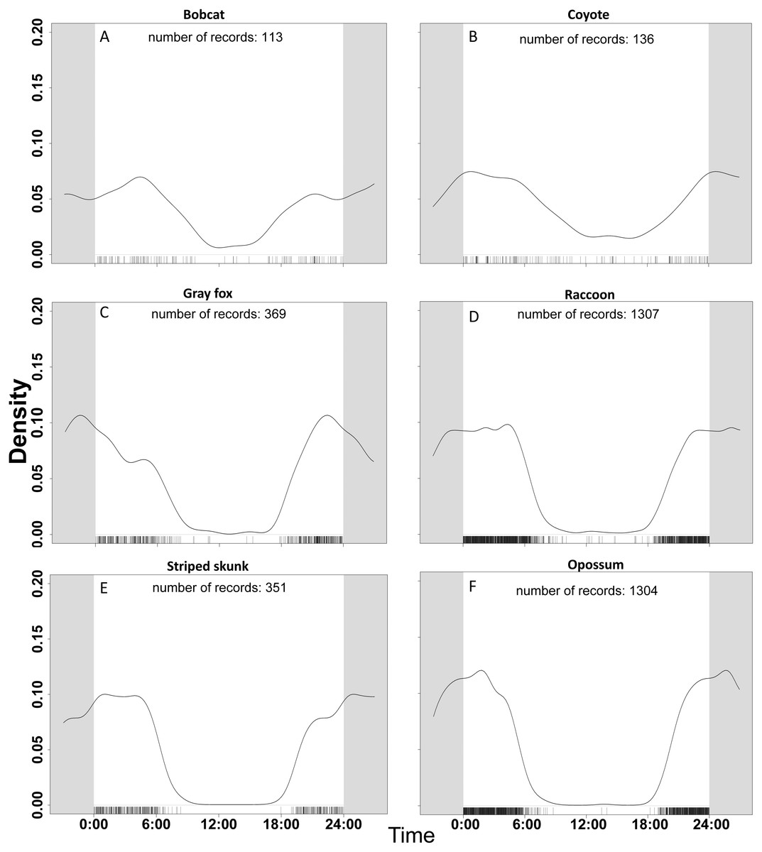
Figure 2: Temporal activity of six species based on data from 47 camera trap sites in and near Corvallis, OR, April 2018–February 2019.
Comparisons of activity from 0:00 to 24:00 between (A) bobcat, (B) coyote, (C) gray fox, (D) raccoon, (E) striped skunk, and (F) opossum. Gray area continues the time cycle on either side of 0:00 and 24:00. The number of records reflects the number of detections per species once duplicate events (events within 30 min of each other) were removed. Mesocarnivores in the aggregate were more active during crepuscular and nighttime hours. Larger bodied mesocarnivores (bobcats, coyotes) were more active during the day than smaller bodied species (opossum, gray fox, raccoon, striped skunk).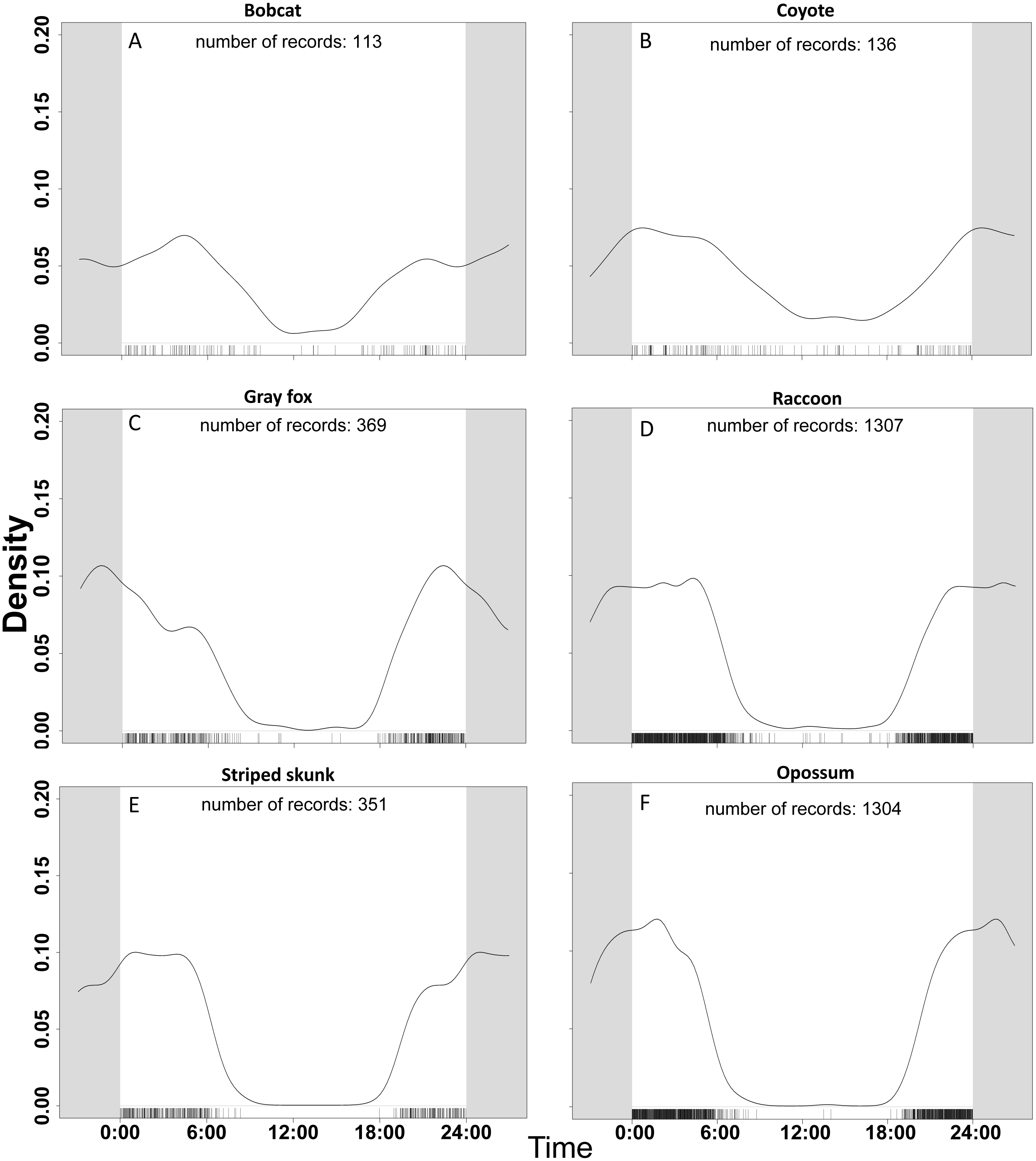
Bobcat
Roads (βONROAD = 1.08 ± 0.25) were the strongest predictor of bobcat detection probability (Appendix A). Based on the most supported bobcat model [Ψ(UC100M+GC100M), p (ONROAD)], bobcat occupancy declined with urban cover (βUC100M = − 1.08 ± 0.43) and increased with grassland cover (βGC100M = 0.79 ± 0.65) at the 100 m scale. The second most-supported model (ΔAICc = 0.23) was the univariate model with urban cover showing a negative association with landscape use (βUC100M = − 1.18 ± 0.41).
Coyote
A negative association with precipitation (βPRECIP = − 0.54 ± 0.12) was our strongest detection model for coyote and was carried forward to the site-level occupancy models. Our strongest occupancy model for coyote [Ψ(USUMRD100M+WC500M), p (PRECIP)], associated increased landscape use with the amount of water cover (streams, lakes, wetlands) within 500 m (βWC500M = 0.73 ± 0.39) and the density of unpaved roads within 100 m (βUSUM100M = 0.79 ± 0.37). The second-ranked (ΔAICc = 0.85) model [Ψ(WC500M+FC100M), p (PRECIP)] indicated increased use of areas with higher amounts of forest cover within 100 m (βFC100M = 0.74 ± 0.37). We also found the positive use relationships with water, unpaved roads, and forest cover in our third strongest (ΔAICc = 1.75) model.
Gray fox
Gray fox detection probability was best predicted by roads (βONROAD = − 1.57 ± 0.27). Gray fox landscape use appeared to be most influenced by grassland cover based on our top model [Ψ(GC1000M), p (ONROAD)], which indicated a positive relationship with grassland cover within 1000 m (βGC1000M = 1.19 ± 0.42). Our top models also suggested that gray fox landscape use was influenced by paved road density and urban cover (Table 2). The second strongest (ΔAICc = 0.87) model [Ψ(GC1000M+PSUMRD500M), p(ONROAD)] indicated weak support for a negative effect of paved road density (βPSUMRD500M = − 0.47 ± 0.38). Our model that included urban cover (ΔAICc = 2.50) [Ψ(GC1000M+UC500M), p (ONROAD)] showed that there was no clear effect on landscape use by urban cover (βUC500M = − 0.034 ± 0.350).
Opossum
Temperature (βTEMP = 0.21 ± 0.07) was the strongest detection model for opossum, providing a more supported model than precipitation (βPRECIP = − 0.11 ± 0.06) and the placement of cameras on roads (βONROAD = − 0.09 ± 0.23). The strongest occupancy model [Ψ(rDTSTRUC), p (TEMP)] suggests that opossum occupancy probability declines as distance to human structure increases (βDTSTRUC = − 1.78 ± 0.66) (Table 2). The model with the next most support (ΔAICc = 0.15) [Ψ(DTSTRUC+UC100M), p (TEMP)] showed that urban cover (βUC100M = 0.80 ± 0.57) also had a positive relationship with opossum occupancy, as well as reaffirming the previous model’s influence of human structures (βDTSTRUC = − 1.20 ± 0.62). Models for unpaved roads (ΔAICc = 0.47) [Ψ(USUMRD500M), p (TEMP)] and forest cover (ΔAICc = 0.51) [Ψ(FC100M), p (TEMP)] also showed to influence opossum landscape use. Both unpaved roads (βUSUMRD500M = − 1.32 ± 0.41) and forest cover (βFC100M = − 1.32 ± 0.40) had a negative relationship to opossum occupancy.
Raccoon
Our top racoon detection models suggested that roads negatively impacted detection (βONROAD = − 2.80 ± 0.40) and had a greater magnitude of effect than precipitation (βPRECIP = 0.06 ± 0.06) or temperature (βTEMP = − 0.1 ± 0.06). The strongest raccoon occupancy model was a univariate model [Ψ(rDTSTRUC), p (ONROAD)] with landscape use decreasing as distance to human structures increased (βDTSTRUC = − 1.57 ± 0.63) (Table 2). The second most supported (ΔAICc = 2.05) [Ψ(DTSTRUC+PSUMRD100M), p (ONROAD)] model indicated a weak positive relationship with paved road density (βPSUMRD100M = 0.31 ± 0.47) along with a strong positive relationship between raccoon occupancy and human structures (βDTSTRUC = − 1.32 ± 0.69) (Table 2).
Striped skunk
The most supported detection model for striped skunk included a negative effect of camera placement on roads (βONROAD = − 0.67 ± 0.22), which we carried forward and used with all subsequent landscape occupancy models. The most supported use model [Ψ(FC500M), p(ONROAD)] for striped skunk included the positive effect of forest cover at 500 m (βFC500M = 0.8753 ± 0.3370) (Table 2). The second strongest model (ΔAICc = 1.84), [Ψ(PSUMRD100M), p (ONROAD)], indicated a negative effect of paved road density at 100 m (βSUMRD1000M = − 0.8250 ± 0.3804). The third strongest model (ΔAICc = 2.06) [Ψ(UC1000M), p (ONROAD)] included negative relationship to urban cover at the 1000 m scale, (βUC1000M = − 0.82 ± 0.39).
Discussion
We explored mesopredator occupancy in human-dominated landscapes across a gradient of urban, rural, and forested environments. Mammalian carnivores can be sensitive to urbanization and have varying responses along an urban to rural gradient (Goad et al., 2014; Salek, Drahnikova & Tkadlec, 2015; Wang, Allen & Wilmers, 2015). The species-level responses to anthropogenic disturbance varied tremendously, with some species being human exploiters tied to urban cover, others being human adapters that were neither positively nor negatively affected by disturbance and agriculture, and human avoider species that were negatively associated with anthropogenic landscape features. The individual species results of our study were largely supported by some established literature from other regions. However, some of our results were contradictory to expectations based on previous research. For example, we found that grassland cover was a more important landscape feature than forest cover for both bobcat and gray fox, whereas in other studies, forest cover was a better predictor of landscape use (Tucker, Clark & Gosselink, 2008; Lesmeister et al., 2015). We found that raccoon and opossum were human exploiters, and in contrast to other studies, striped skunk landscape use was negatively associated with urban development.
We were able to identify opossum and raccoon as human exploiters due to their high use of urban cover and areas near structures (Fig. 3, Table 2). Opossum was common in both urban and rural developments, had negative relationships with forested cover, and increased use in areas with high urban cover density, suggesting that they can exploit much more densely populated areas than other species. Similarly, raccoon occupancy was greatest in urban areas and lowest in forested sites. This is consistent with previous results suggesting that opossum (Markovchick-Nicholls et al., 2008; Wright, Burt & Jackson, 2012) and raccoon (Prange, Gehrt & Wiggers, 2003; Prange, Gehrt & Wiggers, 2004) are competent cohabiters with humans that exploit urban areas. Although we do not have direct data on their population density, the patterns of occupancy that we observed strongly suggest that raccoon and opossum population density is substantially higher in urban areas. The occupancy of opossum and raccoon was strongly associated with human structures, and opossum was positively associated with urban cover even when accounting for proximity to human structures (Table 2). Similarly, opossum had a substantially stronger negative relationship with forest cover, suggesting that raccoon, unlike opossum, were not actively avoiding forested areas (Table 2). Collectively, these results suggest that while both species are associated with humans, opossum have greater affinity for urban environments. Presumably that affinity for urban environments is due to a combination of anthropogenic subsidies (Bozek, Prange & Gehrt, 2007) and reduced predation risk from larger predators (Lesmeister et al., 2015). The association of raccoon and opossum with urban environments was expected, but we did not find the predicted association with natural water sources that was found by others to be an important predictor of opossum and raccoon occupancy (Stuewer, 1943; Gehrt & Fritzell, 1998; Gehrt & Fritzell, 1999; Fidino, Lehrer & Magle, 2016). However, Fidino, Lehrer & Magle (2016) also noted that anthropogenic water sources may allow opossum to colonize previously uninhabitable urban patches. We did not include small human-derived water sources as a covariate in our models because they can be ephemeral and not detectable in land cover databases.
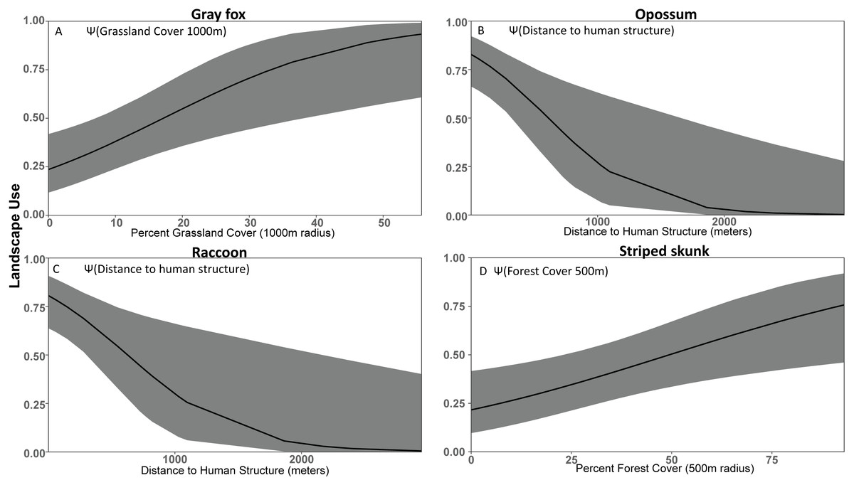
Figure 3: Covariate effect size plots for species with univariate models based on data from 47 camera trap sites in and near Corvallis, OR, April 2018–February 2019.
Landscape use of (A) gray fox, (B) opossum, (C) raccoon, and (D) striped skunk using the most supported occupancy model for each respective species. The black line represents the use estimate while the shaded area represents the upper and lower confidence intervals.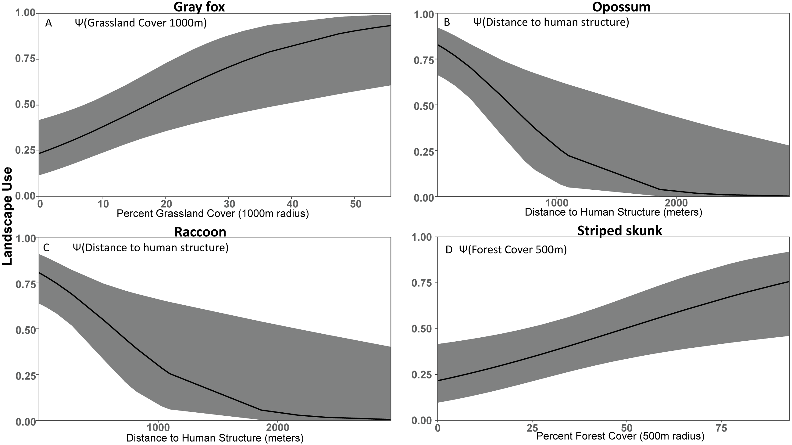
We expected striped skunk to be a human adapted species; but our results suggest that they are human avoiders with higher use of forest cover and low use of human development. Our findings are similar to some studies (Stout & Sonenshine, 1974; Bixler & Gittleman, 2000), but differ from other studies that found striped skunk home ranges oriented along roads and levees and that this species associates with structures for resting and denning (Frey & Conover, 2006; Theimer et al., 2017). Our study area experiences less volatile temperatures compared to those in the study areas of Frey & Conover (2006) and Theimer et al. (2017), which may mean less incentive to use human structures to help in thermoregulation. Dissuading depredation from larger species by their defense mechanism and warning coloration (Walton & Larivière, 1994; Fisher & Stankowich, 2018) may also make forested cover more viable for striped skunk compared to species of similar body size.
As expected based on previous studies (Lesmeister et al., 2015), bobcat tended to be human avoiders in this study with a negative association with urban cover (Fig. 4). Previous studies have shown that when bobcat inhabit urbanized areas their home ranges consist primarily of natural areas (Riley et al., 2003; Riley, 2006). Bobcat appear to decline in response to increasing urbanization proximity and intensity (Tigas, Van Vuren & Sauvajot, 2002; George & Crooks, 2006; Ordeñana et al., 2010). Crooks (2002) suggests that bobcat appear to be particularly sensitive to fragmentation and the probability of bobcat occurrence is greater in larger reserves. In George & Crooks (2006) bobcat was less likely to be detected on cameras with high human activity. Cameras we placed in the Macdonald-Dunn Research Forest were on trails or roads that were commonly frequented by humans. If bobcat was avoiding areas with human activity, we may have observed a greater association with forest cover if we surveyed more forest sites away from human-use areas. We noted that while bobcat use was greater in less developed areas there were some detections in highly developed areas, although these events were infrequent similar to that of Goad et al. (2014).
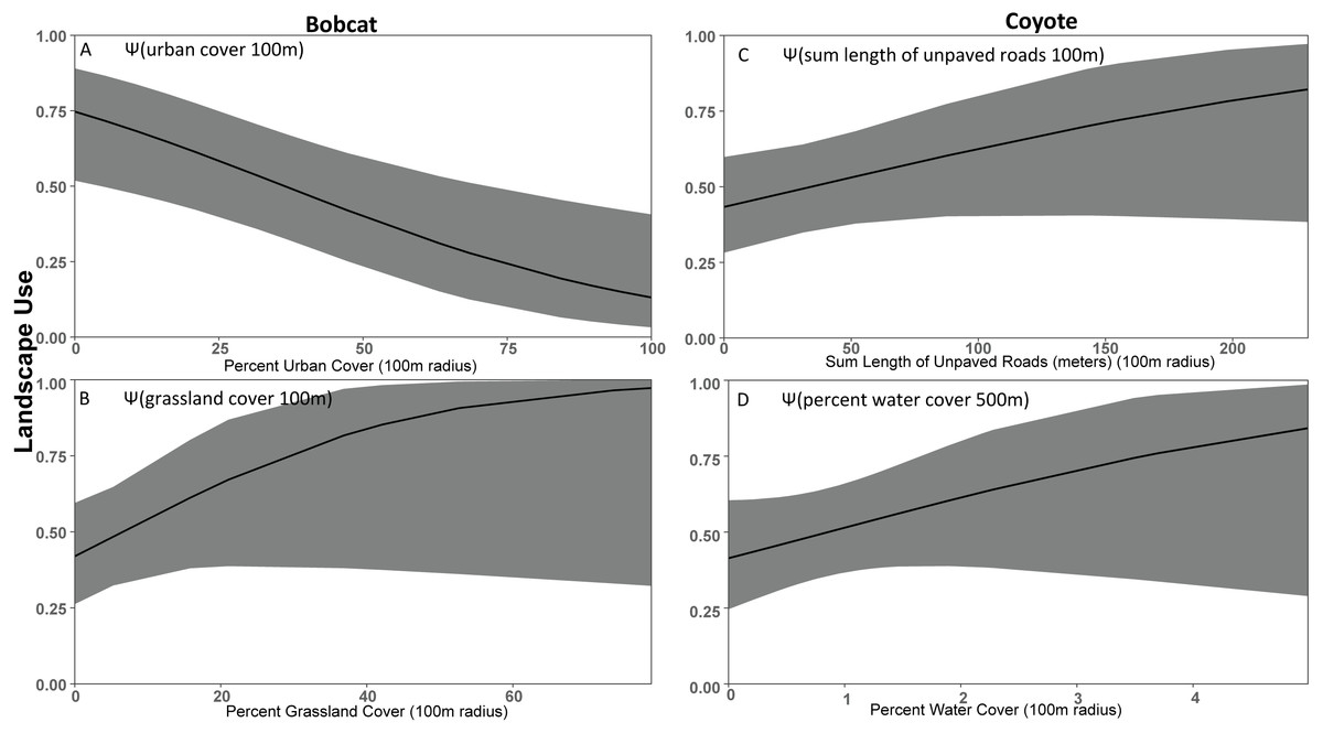
Figure 4: Covariate effect size plots for species with multivariate models based on data from 47 camera trap sites in and near Corvallis, OR, April 2018–February 2019.
Bobcat landscape use based on urban cover at the 100 m scale (A) and grassland cover at the 100 m scale (B) and coyote landscape use on sum of unpaved roads at the 100 m scale (C) and water cover at the 100 m scale (D). The black line represents the use estimate while the shaded area represents the upper and lower confidence intervals.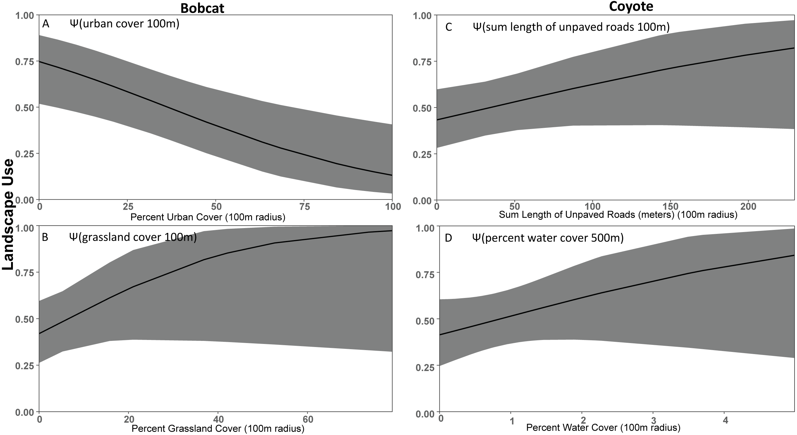
Our results did not support our prediction that coyote would be human avoiders. Rather, our results suggest that coyote preferred natural areas like grassland and water cover, and urban features had little effect. Thusly, it was difficult to define coyote as solely human avoiders or exploiters, so we classified them as human adapters. We found that coyote were positively associated with unpaved roads, suggesting modest association with the lightest form of anthropogenic disturbance, but coyote was also positively associated with water and forest cover. Other studies have shown coyote frequently exploit urban environments due to their ability to take advantage of anthropogenic features for food, water, and shelter (Chamberlain, Lovell & Leopold, 2000; Kays, Gompper & Ray, 2008; Gehrt, Riley & Cypher, 2010). However, previous research also suggests that coyote need core wildland habitats (Grinder & Krausman, 2001; Gehrt, Anchor & White, 2009). There was modest support that forest cover was a positive predictor for coyote use, but that effect was less important than we predicted when compared to other covariates such as water cover (Riley et al., 2003; Tucker, Clark & Gosselink, 2008; Gehrt, Anchor & White, 2009; Magle et al., 2014).
In our study area, gray fox appeared to be neither strictly human exploiters nor avoiders. Following the precedent set by our coyote results and classification, we classified gray fox as human adapters. In the literature, there are conflicting gray fox results across various landscapes about how the species is positioned on the exploiter-avoider continuum. Results from Riley (2006) suggest that gray fox reach higher densities in and around urbanized areas, whereas Markovchick-Nicholls et al. (2008) found that gray fox were negatively associated with roads, much like our results. Lesmeister et al. (2015) noted that landscape use of gray fox may be driven by both interference competition by bobcat and coyote and the availability of small mammal prey. Our results suggested a negative relationship with human developments, but the support is weak enough that we did not feel it would be appropriate to classify this species as a human avoider in this study area. In contrast to results from Lesmeister et al. (2015), we found no evidence that forest cover was a significant predictor for gray fox occurrence, in either direction, but in our study area, free-ranging dogs were not as prevalent as in southern Illinois, which may have a depressing effect on gray fox landscape use (Morin et al., 2018). We observed that grassland cover was positively associated with gray fox occurrence, and previous studies found increased abundance of gray fox in areas with high levels of fragmentation of forested and grassland cover (Fuller & Cypher, 2004; Cooper, Nielsen & McDonald, 2012). Corvallis and the surrounding landscape have moderate levels of fragmentation from urban development, timber harvesting, and agricultural fields.
We have characterized the habitat associations of mesocarnivores, but mesocarnivore occupancy can also be influenced by competition and predation. We would be remiss to overlook the importance of cougars as the apex predator in carnivore communities. Throughout our survey effort, there were only 30 detections of cougar, and they were largely confined to the MacDonald-Dunn Research Forest. Based on previous studies (Chamberlain, Lovell & Leopold, 2000; O’connell et al., 2006; Cove et al., 2012; Lesmeister et al., 2015; Gompper et al., 2016), we expected forest cover to be a stronger predictor of landscape occupancy for mesopredators, but many of these studies occurred in areas without cougar where forested areas posed less risk. Species interactions with coyote may also be influencing the distribution of gray fox, which appear to be avoiding forested areas where coyote were more common to reduce intraguild conflict and interference competition (Temple, Chamberlain & Conner, 2010; Levi & Wilmers, 2012; Lesmeister et al., 2015). In another urban-rural carnivore study, raccoon distribution was negatively affected by coyote distribution while being positively correlated with predictors such as road density and distance to urban center (Randa & Yunger, 2006).
Our findings supported the predictions that mesopredators would have limited activity during daylight hours. Previous studies have also documented increased nocturnal activity by mesocarnivores (Riley et al., 2003; Wang, Allen & Wilmers, 2015). There appears to be a distinction between the activity patterns of species that preferred natural areas versus urban areas. However, we were unable to determine if this was primarily driven by body size or human activity, or if both were contributing factors. Both bobcat and coyote appeared to keep their circadian patterns as detections of them were common around dawn and dusk. Species with the most urban use, raccoon and opossum, showed less daytime activity (0600-1800) presumably to avoid increased human activity in these areas during these hours. Many studies (Larivière & Messier, 1998; Neiswenter, Dowler & Young, 2010) have documented the nocturnal nature of striped skunk, and that was reflected in our results as well.
Conclusions
As urbanization continues, it is important to understand how a species might respond to increased urban development and the factors that might put a species at increased risk of decline to avoid the decline of once-common carnivores that has been observed in other species (Purvis et al., 2000; Gompper & Hackett, 2005; Gaston & Fuller, 2007). The taxa in this study have large ranges spanning much of North America, yet it is common for studies in different regions to observe a variety of species-specific relationships with land cover and human development. We provide information on how some common mesocarnivores use landscapes across a gradient of urban to rural to forested environments in the context of the vertebrate community and forest type of the mesic Pacific Northwest forest of the United States. Our results differed from several studies of this guild in other regions of North America, highlighting the importance of ecological context for landscape use along a gradient of urban to natural land cover. The level of human tolerance and species interactions may have also influenced our observed landscape use. For example, gray fox was typically associated with forest and grassland cover, but competitors such as bobcat (Lesmeister et al., 2015) and interference competition in areas of high coyote abundance can influence gray fox distribution (Crooks, 2002; Farias et al., 2005; Temple, Chamberlain & Conner, 2010; Ordeñana et al., 2010). Our results inform how mesopredator communities respond to anthropogenic disturbance in a distinct context, which together with other research can help elucidate the mechanisms underlying their observed distributions and inform their conservation and management. Management actions that impact these species are likely to be most effective if based on locally derived information.
Supplemental Information
Site and survey level covarites across the study area in and near Corvallis, OR, April 2018 - February 2019
Covaraite values (forest, water, urban cover, etc.) of each site along with the temperature and precipitation data during the survey period.
Binary detection histories for species in the Corvallis, OR, study area April 2018 - February 2019
Weekly binary detection histories for deer, coyote, cougar, domestic cat, domestic dog, gray fox, human, opossum, raccoon, and striped skunk.
Species detection histories for activity analysis.
Date and time data for deer, coyote, cougar, domestic cat, domestic dog, gray fox, human, opossum, raccoon, and striped skunk.
Detection and occupancy code for for the species of interest with PRESENCE output files
R version 3.53 (2019-03-11) used to run the provided code. ’RPresence’ version 2.12.27. ’ggplot2′version 3.3.1.
Evaluation of survey covariates related to detection probabilities (p) for bobcats, coyotes, gray foxes, opossums, raccoons, and striped skunks in and near Corvallis, OR, April 2018 –February 2019
To estimate p for each species, we held the occupancy parameter constant and fit encounter history data from 47 camera sites. We included the null (.) model for each species for assessment of relative strength of survey covariates to explain heterogeneity in detection probabilities.
Occupancy ( Ψ) model results from Single-Species Single-Season Models for bobcats, coyotes, gray foxes, opossums, raccoons, and striped skunks in and near Corvallis, OR, April 2018 –February 2019
To estimate Ψ for each species, we used the detection parameter that was most supported for the respective species and fit encounter history data from 47 camera sites.